10.1 Panel Data
Key Concept 10.1
Notation for Panel Data
In contrast to cross-section data where we have observations on \(n\) subjects (entities), panel data has observations on \(n\) entities at \(T\geq2\) time periods. This is denoted as
\[(X_{it},Y_{it}), \ i=1,\dots,n \ \ \ \text{and} \ \ \ t=1,\dots,T \] where the index \(i\) refers to the entity while \(t\) refers to the time period.
Sometimes panel data is also called longitudinal data as it adds a temporal dimension to cross-sectional data. Let us have a look at the dataset Fatalities by checking its structure and listing the first few observations.
# load the packagees and the dataset
library(AER)
library(plm)
data(Fatalities)
# pdata.frame() declares the data as panel data.
Fatalities<- pdata.frame(Fatalities, index = c("state", "year"))
# obtain the dimension and inspect the structure
is.data.frame(Fatalities)
#> [1] TRUE
dim(Fatalities)
#> [1] 336 34str(Fatalities)
#> Classes 'pdata.frame' and 'data.frame': 336 obs. of 34 variables:
#> $ state : Factor w/ 48 levels "al","az","ar",..: 1 1 1 1 1 1 1 2 2 2 ...
#> ..- attr(*, "names")= chr [1:336] "al-1982" "al-1983" "al-1984" "al-1985" ...
#> ..- attr(*, "index")=Classes 'pindex' and 'data.frame': 336 obs. of 2 variables:
#> .. ..$ state: Factor w/ 48 levels "al","az","ar",..: 1 1 1 1 1 1 1 2 2 2 ...
#> .. ..$ year : Factor w/ 7 levels "1982","1983",..: 1 2 3 4 5 6 7 1 2 3 ...
#> $ year : Factor w/ 7 levels "1982","1983",..: 1 2 3 4 5 6 7 1 2 3 ...
#> ..- attr(*, "names")= chr [1:336] "al-1982" "al-1983" "al-1984" "al-1985" ...
#> ..- attr(*, "index")=Classes 'pindex' and 'data.frame': 336 obs. of 2 variables:
#> .. ..$ state: Factor w/ 48 levels "al","az","ar",..: 1 1 1 1 1 1 1 2 2 2 ...
#> .. ..$ year : Factor w/ 7 levels "1982","1983",..: 1 2 3 4 5 6 7 1 2 3 ...
#> $ spirits : 'pseries' Named num 1.37 1.36 1.32 1.28 1.23 ...
#> ..- attr(*, "names")= chr [1:336] "al-1982" "al-1983" "al-1984" "al-1985" ...
#> ..- attr(*, "index")=Classes 'pindex' and 'data.frame': 336 obs. of 2 variables:
#> .. ..$ state: Factor w/ 48 levels "al","az","ar",..: 1 1 1 1 1 1 1 2 2 2 ...
#> .. ..$ year : Factor w/ 7 levels "1982","1983",..: 1 2 3 4 5 6 7 1 2 3 ...
#> $ unemp : 'pseries' Named num 14.4 13.7 11.1 8.9 9.8 ...
#> ..- attr(*, "names")= chr [1:336] "al-1982" "al-1983" "al-1984" "al-1985" ...
#> ..- attr(*, "index")=Classes 'pindex' and 'data.frame': 336 obs. of 2 variables:
#> .. ..$ state: Factor w/ 48 levels "al","az","ar",..: 1 1 1 1 1 1 1 2 2 2 ...
#> .. ..$ year : Factor w/ 7 levels "1982","1983",..: 1 2 3 4 5 6 7 1 2 3 ...
#> $ income : 'pseries' Named num 10544 10733 11109 11333 11662 ...
#> ..- attr(*, "names")= chr [1:336] "al-1982" "al-1983" "al-1984" "al-1985" ...
#> ..- attr(*, "index")=Classes 'pindex' and 'data.frame': 336 obs. of 2 variables:
#> .. ..$ state: Factor w/ 48 levels "al","az","ar",..: 1 1 1 1 1 1 1 2 2 2 ...
#> .. ..$ year : Factor w/ 7 levels "1982","1983",..: 1 2 3 4 5 6 7 1 2 3 ...
#> $ emppop : 'pseries' Named num 50.7 52.1 54.2 55.3 56.5 ...
#> ..- attr(*, "names")= chr [1:336] "al-1982" "al-1983" "al-1984" "al-1985" ...
#> ..- attr(*, "index")=Classes 'pindex' and 'data.frame': 336 obs. of 2 variables:
#> .. ..$ state: Factor w/ 48 levels "al","az","ar",..: 1 1 1 1 1 1 1 2 2 2 ...
#> .. ..$ year : Factor w/ 7 levels "1982","1983",..: 1 2 3 4 5 6 7 1 2 3 ...
#> $ beertax : 'pseries' Named num 1.54 1.79 1.71 1.65 1.61 ...
#> ..- attr(*, "names")= chr [1:336] "al-1982" "al-1983" "al-1984" "al-1985" ...
#> ..- attr(*, "index")=Classes 'pindex' and 'data.frame': 336 obs. of 2 variables:
#> .. ..$ state: Factor w/ 48 levels "al","az","ar",..: 1 1 1 1 1 1 1 2 2 2 ...
#> .. ..$ year : Factor w/ 7 levels "1982","1983",..: 1 2 3 4 5 6 7 1 2 3 ...
#> $ baptist : 'pseries' Named num 30.4 30.3 30.3 30.3 30.3 ...
#> ..- attr(*, "names")= chr [1:336] "al-1982" "al-1983" "al-1984" "al-1985" ...
#> ..- attr(*, "index")=Classes 'pindex' and 'data.frame': 336 obs. of 2 variables:
#> .. ..$ state: Factor w/ 48 levels "al","az","ar",..: 1 1 1 1 1 1 1 2 2 2 ...
#> .. ..$ year : Factor w/ 7 levels "1982","1983",..: 1 2 3 4 5 6 7 1 2 3 ...
#> $ mormon : 'pseries' Named num 0.328 0.343 0.359 0.376 0.393 ...
#> ..- attr(*, "names")= chr [1:336] "al-1982" "al-1983" "al-1984" "al-1985" ...
#> ..- attr(*, "index")=Classes 'pindex' and 'data.frame': 336 obs. of 2 variables:
#> .. ..$ state: Factor w/ 48 levels "al","az","ar",..: 1 1 1 1 1 1 1 2 2 2 ...
#> .. ..$ year : Factor w/ 7 levels "1982","1983",..: 1 2 3 4 5 6 7 1 2 3 ...
#> $ drinkage : 'pseries' Named num 19 19 19 19.7 21 ...
#> ..- attr(*, "names")= chr [1:336] "al-1982" "al-1983" "al-1984" "al-1985" ...
#> ..- attr(*, "index")=Classes 'pindex' and 'data.frame': 336 obs. of 2 variables:
#> .. ..$ state: Factor w/ 48 levels "al","az","ar",..: 1 1 1 1 1 1 1 2 2 2 ...
#> .. ..$ year : Factor w/ 7 levels "1982","1983",..: 1 2 3 4 5 6 7 1 2 3 ...
#> $ dry : 'pseries' Named num 25 23 24 23.6 23.5 ...
#> ..- attr(*, "names")= chr [1:336] "al-1982" "al-1983" "al-1984" "al-1985" ...
#> ..- attr(*, "index")=Classes 'pindex' and 'data.frame': 336 obs. of 2 variables:
#> .. ..$ state: Factor w/ 48 levels "al","az","ar",..: 1 1 1 1 1 1 1 2 2 2 ...
#> .. ..$ year : Factor w/ 7 levels "1982","1983",..: 1 2 3 4 5 6 7 1 2 3 ...
#> $ youngdrivers: 'pseries' Named num 0.212 0.211 0.211 0.211 0.213 ...
#> ..- attr(*, "names")= chr [1:336] "al-1982" "al-1983" "al-1984" "al-1985" ...
#> ..- attr(*, "index")=Classes 'pindex' and 'data.frame': 336 obs. of 2 variables:
#> .. ..$ state: Factor w/ 48 levels "al","az","ar",..: 1 1 1 1 1 1 1 2 2 2 ...
#> .. ..$ year : Factor w/ 7 levels "1982","1983",..: 1 2 3 4 5 6 7 1 2 3 ...
#> $ miles : 'pseries' Named num 7234 7836 8263 8727 8953 ...
#> ..- attr(*, "names")= chr [1:336] "al-1982" "al-1983" "al-1984" "al-1985" ...
#> ..- attr(*, "index")=Classes 'pindex' and 'data.frame': 336 obs. of 2 variables:
#> .. ..$ state: Factor w/ 48 levels "al","az","ar",..: 1 1 1 1 1 1 1 2 2 2 ...
#> .. ..$ year : Factor w/ 7 levels "1982","1983",..: 1 2 3 4 5 6 7 1 2 3 ...
#> $ breath : Factor w/ 2 levels "no","yes": 1 1 1 1 1 1 1 1 1 1 ...
#> ..- attr(*, "names")= chr [1:336] "al-1982" "al-1983" "al-1984" "al-1985" ...
#> ..- attr(*, "index")=Classes 'pindex' and 'data.frame': 336 obs. of 2 variables:
#> .. ..$ state: Factor w/ 48 levels "al","az","ar",..: 1 1 1 1 1 1 1 2 2 2 ...
#> .. ..$ year : Factor w/ 7 levels "1982","1983",..: 1 2 3 4 5 6 7 1 2 3 ...
#> $ jail : Factor w/ 2 levels "no","yes": 1 1 1 1 1 1 1 2 2 2 ...
#> ..- attr(*, "names")= chr [1:336] "al-1982" "al-1983" "al-1984" "al-1985" ...
#> ..- attr(*, "index")=Classes 'pindex' and 'data.frame': 336 obs. of 2 variables:
#> .. ..$ state: Factor w/ 48 levels "al","az","ar",..: 1 1 1 1 1 1 1 2 2 2 ...
#> .. ..$ year : Factor w/ 7 levels "1982","1983",..: 1 2 3 4 5 6 7 1 2 3 ...
#> $ service : Factor w/ 2 levels "no","yes": 1 1 1 1 1 1 1 2 2 2 ...
#> ..- attr(*, "names")= chr [1:336] "al-1982" "al-1983" "al-1984" "al-1985" ...
#> ..- attr(*, "index")=Classes 'pindex' and 'data.frame': 336 obs. of 2 variables:
#> .. ..$ state: Factor w/ 48 levels "al","az","ar",..: 1 1 1 1 1 1 1 2 2 2 ...
#> .. ..$ year : Factor w/ 7 levels "1982","1983",..: 1 2 3 4 5 6 7 1 2 3 ...
#> $ fatal : 'pseries' Named int 839 930 932 882 1081 1110 1023 724 675 869 ...
#> ..- attr(*, "names")= chr [1:336] "al-1982" "al-1983" "al-1984" "al-1985" ...
#> ..- attr(*, "index")=Classes 'pindex' and 'data.frame': 336 obs. of 2 variables:
#> .. ..$ state: Factor w/ 48 levels "al","az","ar",..: 1 1 1 1 1 1 1 2 2 2 ...
#> .. ..$ year : Factor w/ 7 levels "1982","1983",..: 1 2 3 4 5 6 7 1 2 3 ...
#> $ nfatal : 'pseries' Named int 146 154 165 146 172 181 139 131 112 149 ...
#> ..- attr(*, "names")= chr [1:336] "al-1982" "al-1983" "al-1984" "al-1985" ...
#> ..- attr(*, "index")=Classes 'pindex' and 'data.frame': 336 obs. of 2 variables:
#> .. ..$ state: Factor w/ 48 levels "al","az","ar",..: 1 1 1 1 1 1 1 2 2 2 ...
#> .. ..$ year : Factor w/ 7 levels "1982","1983",..: 1 2 3 4 5 6 7 1 2 3 ...
#> $ sfatal : 'pseries' Named int 99 98 94 98 119 114 89 76 60 81 ...
#> ..- attr(*, "names")= chr [1:336] "al-1982" "al-1983" "al-1984" "al-1985" ...
#> ..- attr(*, "index")=Classes 'pindex' and 'data.frame': 336 obs. of 2 variables:
#> .. ..$ state: Factor w/ 48 levels "al","az","ar",..: 1 1 1 1 1 1 1 2 2 2 ...
#> .. ..$ year : Factor w/ 7 levels "1982","1983",..: 1 2 3 4 5 6 7 1 2 3 ...
#> $ fatal1517 : 'pseries' Named int 53 71 49 66 82 94 66 40 40 51 ...
#> ..- attr(*, "names")= chr [1:336] "al-1982" "al-1983" "al-1984" "al-1985" ...
#> ..- attr(*, "index")=Classes 'pindex' and 'data.frame': 336 obs. of 2 variables:
#> .. ..$ state: Factor w/ 48 levels "al","az","ar",..: 1 1 1 1 1 1 1 2 2 2 ...
#> .. ..$ year : Factor w/ 7 levels "1982","1983",..: 1 2 3 4 5 6 7 1 2 3 ...
#> $ nfatal1517 : 'pseries' Named int 9 8 7 9 10 11 8 7 7 8 ...
#> ..- attr(*, "names")= chr [1:336] "al-1982" "al-1983" "al-1984" "al-1985" ...
#> ..- attr(*, "index")=Classes 'pindex' and 'data.frame': 336 obs. of 2 variables:
#> .. ..$ state: Factor w/ 48 levels "al","az","ar",..: 1 1 1 1 1 1 1 2 2 2 ...
#> .. ..$ year : Factor w/ 7 levels "1982","1983",..: 1 2 3 4 5 6 7 1 2 3 ...
#> $ fatal1820 : 'pseries' Named int 99 108 103 100 120 127 105 81 83 118 ...
#> ..- attr(*, "names")= chr [1:336] "al-1982" "al-1983" "al-1984" "al-1985" ...
#> ..- attr(*, "index")=Classes 'pindex' and 'data.frame': 336 obs. of 2 variables:
#> .. ..$ state: Factor w/ 48 levels "al","az","ar",..: 1 1 1 1 1 1 1 2 2 2 ...
#> .. ..$ year : Factor w/ 7 levels "1982","1983",..: 1 2 3 4 5 6 7 1 2 3 ...
#> $ nfatal1820 : 'pseries' Named int 34 26 25 23 23 31 24 16 19 34 ...
#> ..- attr(*, "names")= chr [1:336] "al-1982" "al-1983" "al-1984" "al-1985" ...
#> ..- attr(*, "index")=Classes 'pindex' and 'data.frame': 336 obs. of 2 variables:
#> .. ..$ state: Factor w/ 48 levels "al","az","ar",..: 1 1 1 1 1 1 1 2 2 2 ...
#> .. ..$ year : Factor w/ 7 levels "1982","1983",..: 1 2 3 4 5 6 7 1 2 3 ...
#> $ fatal2124 : 'pseries' Named int 120 124 118 114 119 138 123 96 80 123 ...
#> ..- attr(*, "names")= chr [1:336] "al-1982" "al-1983" "al-1984" "al-1985" ...
#> ..- attr(*, "index")=Classes 'pindex' and 'data.frame': 336 obs. of 2 variables:
#> .. ..$ state: Factor w/ 48 levels "al","az","ar",..: 1 1 1 1 1 1 1 2 2 2 ...
#> .. ..$ year : Factor w/ 7 levels "1982","1983",..: 1 2 3 4 5 6 7 1 2 3 ...
#> $ nfatal2124 : 'pseries' Named int 32 35 34 45 29 30 25 36 17 33 ...
#> ..- attr(*, "names")= chr [1:336] "al-1982" "al-1983" "al-1984" "al-1985" ...
#> ..- attr(*, "index")=Classes 'pindex' and 'data.frame': 336 obs. of 2 variables:
#> .. ..$ state: Factor w/ 48 levels "al","az","ar",..: 1 1 1 1 1 1 1 2 2 2 ...
#> .. ..$ year : Factor w/ 7 levels "1982","1983",..: 1 2 3 4 5 6 7 1 2 3 ...
#> $ afatal : 'pseries' Named num 309 342 305 277 361 ...
#> ..- attr(*, "names")= chr [1:336] "al-1982" "al-1983" "al-1984" "al-1985" ...
#> ..- attr(*, "index")=Classes 'pindex' and 'data.frame': 336 obs. of 2 variables:
#> .. ..$ state: Factor w/ 48 levels "al","az","ar",..: 1 1 1 1 1 1 1 2 2 2 ...
#> .. ..$ year : Factor w/ 7 levels "1982","1983",..: 1 2 3 4 5 6 7 1 2 3 ...
#> $ pop : 'pseries' Named num 3942002 3960008 3988992 4021008 4049994 ...
#> ..- attr(*, "names")= chr [1:336] "al-1982" "al-1983" "al-1984" "al-1985" ...
#> ..- attr(*, "index")=Classes 'pindex' and 'data.frame': 336 obs. of 2 variables:
#> .. ..$ state: Factor w/ 48 levels "al","az","ar",..: 1 1 1 1 1 1 1 2 2 2 ...
#> .. ..$ year : Factor w/ 7 levels "1982","1983",..: 1 2 3 4 5 6 7 1 2 3 ...
#> $ pop1517 : 'pseries' Named num 209000 202000 197000 195000 204000 ...
#> ..- attr(*, "names")= chr [1:336] "al-1982" "al-1983" "al-1984" "al-1985" ...
#> ..- attr(*, "index")=Classes 'pindex' and 'data.frame': 336 obs. of 2 variables:
#> .. ..$ state: Factor w/ 48 levels "al","az","ar",..: 1 1 1 1 1 1 1 2 2 2 ...
#> .. ..$ year : Factor w/ 7 levels "1982","1983",..: 1 2 3 4 5 6 7 1 2 3 ...
#> $ pop1820 : 'pseries' Named num 221553 219125 216724 214349 212000 ...
#> ..- attr(*, "names")= chr [1:336] "al-1982" "al-1983" "al-1984" "al-1985" ...
#> ..- attr(*, "index")=Classes 'pindex' and 'data.frame': 336 obs. of 2 variables:
#> .. ..$ state: Factor w/ 48 levels "al","az","ar",..: 1 1 1 1 1 1 1 2 2 2 ...
#> .. ..$ year : Factor w/ 7 levels "1982","1983",..: 1 2 3 4 5 6 7 1 2 3 ...
#> $ pop2124 : 'pseries' Named num 290000 290000 288000 284000 263000 ...
#> ..- attr(*, "names")= chr [1:336] "al-1982" "al-1983" "al-1984" "al-1985" ...
#> ..- attr(*, "index")=Classes 'pindex' and 'data.frame': 336 obs. of 2 variables:
#> .. ..$ state: Factor w/ 48 levels "al","az","ar",..: 1 1 1 1 1 1 1 2 2 2 ...
#> .. ..$ year : Factor w/ 7 levels "1982","1983",..: 1 2 3 4 5 6 7 1 2 3 ...
#> $ milestot : 'pseries' Named num 28516 31032 32961 35091 36259 ...
#> ..- attr(*, "names")= chr [1:336] "al-1982" "al-1983" "al-1984" "al-1985" ...
#> ..- attr(*, "index")=Classes 'pindex' and 'data.frame': 336 obs. of 2 variables:
#> .. ..$ state: Factor w/ 48 levels "al","az","ar",..: 1 1 1 1 1 1 1 2 2 2 ...
#> .. ..$ year : Factor w/ 7 levels "1982","1983",..: 1 2 3 4 5 6 7 1 2 3 ...
#> $ unempus : 'pseries' Named num 9.7 9.6 7.5 7.2 7 ...
#> ..- attr(*, "names")= chr [1:336] "al-1982" "al-1983" "al-1984" "al-1985" ...
#> ..- attr(*, "index")=Classes 'pindex' and 'data.frame': 336 obs. of 2 variables:
#> .. ..$ state: Factor w/ 48 levels "al","az","ar",..: 1 1 1 1 1 1 1 2 2 2 ...
#> .. ..$ year : Factor w/ 7 levels "1982","1983",..: 1 2 3 4 5 6 7 1 2 3 ...
#> $ emppopus : 'pseries' Named num 57.8 57.9 59.5 60.1 60.7 ...
#> ..- attr(*, "names")= chr [1:336] "al-1982" "al-1983" "al-1984" "al-1985" ...
#> ..- attr(*, "index")=Classes 'pindex' and 'data.frame': 336 obs. of 2 variables:
#> .. ..$ state: Factor w/ 48 levels "al","az","ar",..: 1 1 1 1 1 1 1 2 2 2 ...
#> .. ..$ year : Factor w/ 7 levels "1982","1983",..: 1 2 3 4 5 6 7 1 2 3 ...
#> $ gsp : 'pseries' Named num -0.0221 0.0466 0.0628 0.0275 0.0321 ...
#> ..- attr(*, "names")= chr [1:336] "al-1982" "al-1983" "al-1984" "al-1985" ...
#> ..- attr(*, "index")=Classes 'pindex' and 'data.frame': 336 obs. of 2 variables:
#> .. ..$ state: Factor w/ 48 levels "al","az","ar",..: 1 1 1 1 1 1 1 2 2 2 ...
#> .. ..$ year : Factor w/ 7 levels "1982","1983",..: 1 2 3 4 5 6 7 1 2 3 ...
#> - attr(*, "index")=Classes 'pindex' and 'data.frame': 336 obs. of 2 variables:
#> ..$ state: Factor w/ 48 levels "al","az","ar",..: 1 1 1 1 1 1 1 2 2 2 ...
#> ..$ year : Factor w/ 7 levels "1982","1983",..: 1 2 3 4 5 6 7 1 2 3 ...# list the first few observations
head(Fatalities)
#> state year spirits unemp income emppop beertax baptist mormon
#> al-1982 al 1982 1.37 14.4 10544.15 50.69204 1.539379 30.3557 0.32829
#> al-1983 al 1983 1.36 13.7 10732.80 52.14703 1.788991 30.3336 0.34341
#> al-1984 al 1984 1.32 11.1 11108.79 54.16809 1.714286 30.3115 0.35924
#> al-1985 al 1985 1.28 8.9 11332.63 55.27114 1.652542 30.2895 0.37579
#> al-1986 al 1986 1.23 9.8 11661.51 56.51450 1.609907 30.2674 0.39311
#> al-1987 al 1987 1.18 7.8 11944.00 57.50988 1.560000 30.2453 0.41123
#> drinkage dry youngdrivers miles breath jail service fatal nfatal
#> al-1982 19.00 25.0063 0.211572 7233.887 no no no 839 146
#> al-1983 19.00 22.9942 0.210768 7836.348 no no no 930 154
#> al-1984 19.00 24.0426 0.211484 8262.990 no no no 932 165
#> al-1985 19.67 23.6339 0.211140 8726.917 no no no 882 146
#> al-1986 21.00 23.4647 0.213400 8952.854 no no no 1081 172
#> al-1987 21.00 23.7924 0.215527 9166.302 no no no 1110 181
#> sfatal fatal1517 nfatal1517 fatal1820 nfatal1820 fatal2124 nfatal2124
#> al-1982 99 53 9 99 34 120 32
#> al-1983 98 71 8 108 26 124 35
#> al-1984 94 49 7 103 25 118 34
#> al-1985 98 66 9 100 23 114 45
#> al-1986 119 82 10 120 23 119 29
#> al-1987 114 94 11 127 31 138 30
#> afatal pop pop1517 pop1820 pop2124 milestot unempus emppopus
#> al-1982 309.438 3942002 208999.6 221553.4 290000.1 28516 9.7 57.8
#> al-1983 341.834 3960008 202000.1 219125.5 290000.2 31032 9.6 57.9
#> al-1984 304.872 3988992 197000.0 216724.1 288000.2 32961 7.5 59.5
#> al-1985 276.742 4021008 194999.7 214349.0 284000.3 35091 7.2 60.1
#> al-1986 360.716 4049994 203999.9 212000.0 263000.3 36259 7.0 60.7
#> al-1987 368.421 4082999 204999.8 208998.5 258999.8 37426 6.2 61.5
#> gsp
#> al-1982 -0.02212476
#> al-1983 0.04655825
#> al-1984 0.06279784
#> al-1985 0.02748997
#> al-1986 0.03214295
#> al-1987 0.04897637# summarize the variables 'state' and 'year'
summary(Fatalities[, c(1, 2)])
#> state year
#> al : 7 1982:48
#> az : 7 1983:48
#> ar : 7 1984:48
#> ca : 7 1985:48
#> co : 7 1986:48
#> ct : 7 1987:48
#> (Other):294 1988:48We find that the dataset consists of 336 observations on 34 variables. Notice that the variable state is a factor variable with 48 levels (one for each of the 48 contiguous federal states of the U.S.). The variable year is also a factor variable that has 7 levels identifying the time period when the observation was made. This gives us \(7\times48 = 336\) observations in total. Since all variables are observed for all entities and over all time periods, the panel is balanced. If there were missing data for at least one entity in at least one time period we would call the panel unbalanced.
Example: Traffic Deaths and Alcohol Taxes
We start by reproducing Figure 10.1 of the book. To this end we estimate simple regressions using data for years 1982 and 1988 that model the relationship between beer tax (adjusted for 1988 dollars) and the traffic fatality rate, measured as the number of fatalities per 10000 inhabitants. Afterwards, we plot the data and add the corresponding estimated regression functions.
# define the fatality rate
Fatalities$fatal_rate <- Fatalities$fatal / Fatalities$pop * 10000

# subset the data
Fatalities1982 <- subset(Fatalities, year == "1982")
Fatalities1988 <- subset(Fatalities, year == "1988")
# estimate simple regression models using 1982 and 1988 data
fatal1982_mod <- lm(fatal_rate ~ beertax, data = Fatalities1982)
fatal1988_mod <- lm(fatal_rate ~ beertax, data = Fatalities1988)
coeftest(fatal1982_mod, vcov. = vcovHC, type = "HC1")
#>
#> t test of coefficients:
#>
#> Estimate Std. Error t value Pr(>|t|)
#> (Intercept) 2.01038 0.14957 13.4408 <2e-16 ***
#> beertax 0.14846 0.13261 1.1196 0.2687
#> ---
#> Signif. codes: 0 '***' 0.001 '**' 0.01 '*' 0.05 '.' 0.1 ' ' 1
coeftest(fatal1988_mod, vcov. = vcovHC, type = "HC1")
#>
#> t test of coefficients:
#>
#> Estimate Std. Error t value Pr(>|t|)
#> (Intercept) 1.85907 0.11461 16.2205 < 2.2e-16 ***
#> beertax 0.43875 0.12786 3.4314 0.001279 **
#> ---
#> Signif. codes: 0 '***' 0.001 '**' 0.01 '*' 0.05 '.' 0.1 ' ' 1The estimated regression functions are \[\begin{align*} \widehat{FatalityRate} =& \, \underset{(0.15)}{2.01} + \underset{(0.13)}{0.15} \times BeerTax \quad (1982 \text{ data}), \\ \widehat{FatalityRate} =& \, \underset{(0.11)}{1.86} + \underset{(0.13)}{0.44} \times BeerTax \quad (1988 \text{ data}). \end{align*}\]
# plot the observations and add the estimated regression line for 1982 data
plot(x = as.double(Fatalities1982$beertax),
     y = as.double(Fatalities1982$fatal_rate),
     xlab = "Beer tax (in 1988 dollars)",
     ylab = "Fatality rate (fatalities per 10000)",
     main = "Traffic Fatality Rates and Beer Taxes in 1982",
     ylim = c(0, 4.5),
     pch = 20,
     col = "steelblue")

abline(fatal1982_mod, lwd = 1.5, col="darkred")
legend("topright",lty=1,col="darkred","Estimated Regression Line")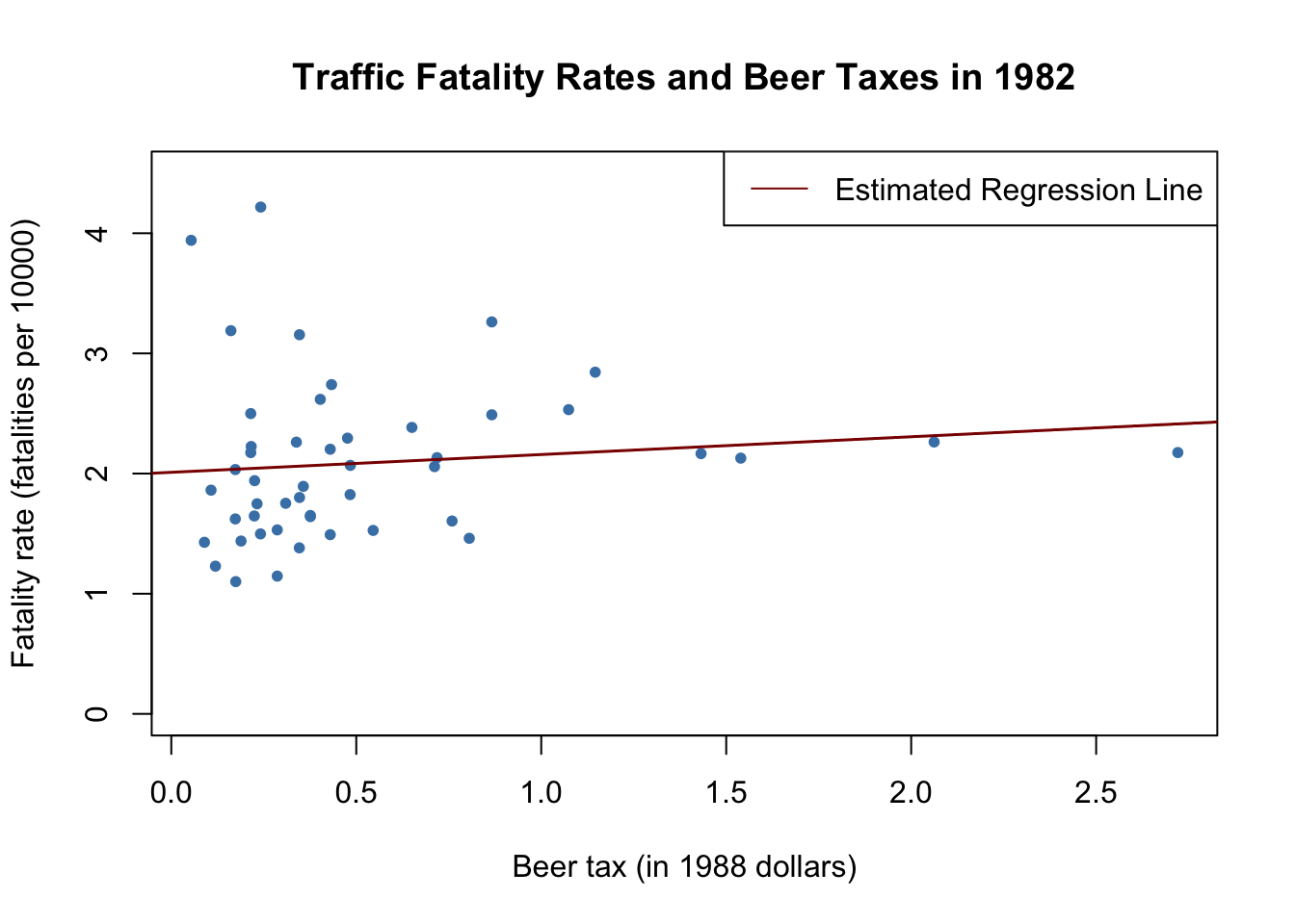
# plot observations and add estimated regression line for 1988 data
plot(x = as.double(Fatalities1988$beertax),
     y = as.double(Fatalities1988$fatal_rate),
     xlab = "Beer tax (in 1988 dollars)",
     ylab = "Fatality rate (fatalities per 10000)",
     main = "Traffic Fatality Rates and Beer Taxes in 1988",
     ylim = c(0, 4.5),
     pch = 20,
     col = "steelblue")

abline(fatal1988_mod, lwd = 1.5,col="darkred")
legend("bottomright",lty=1,col="darkred","Estimated Regression Line")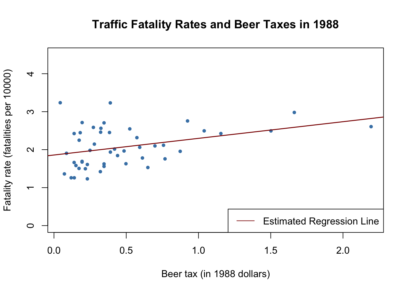
In both plots, each point represents observations of beer tax and fatality rate for a given state in the respective year. The regression results indicate a positive relationship between the beer tax and the fatality rate for both years. The estimated coefficient on beer tax for the 1988 data is almost three times as large as for the 1982 dataset. This is contrary to our expectations: alcohol taxes are supposed to lower the rate of traffic fatalities. As we known from Chapter 6, this is possibly due to omitted variable bias, since both models do not include any covariates, e.g., economic conditions. This could be corrected by using a multiple regression approach. However, this cannot account for omitted unobservable factors that differ from state to state but can be assumed to be constant over the observation span, e.g., the populations’ attitude towards drunk driving. As shown in the next section, panel data allow us to hold such factors constant.