11.1 Binary Dependent Variables and the Linear Probability Model
Key Concept 11.1
The Linear Probability Model
The linear regression model
\[Y_i = \beta_0 + \beta_1 X_{1i} + \beta_2 X_{2i} + \dots + \beta_k X_{ki} + u_i\] with a binary dependent variable \(Y_i\) is called the linear probability model. In the linear probability model we have \[E(Y\vert X_1,X_2,\dots,X_k) = P(Y=1\vert X_1, X_2,\dots, X_3)\] where \[ P(Y = 1 \vert X_1, X_2, \dots, X_k) = \beta_0 + \beta_1 + X_1 + \beta_2 X_2 + \dots + \beta_k X_k.\]
Thus, \(\beta_j\) can be interpreted as the change in the probability that \(Y_i=1\), holding constant the other \(k-1\) regressors. Just as in common multiple regression, the \(\beta_j\) can be estimated using OLS and the robust standard error formulas can be used for hypothesis testing and computation of confidence intervals.
In most linear probability models, \(R^2\) has no meaningful interpretation since the regression line can never fit the data perfectly if the dependent variable is binary and the regressors are continuous. This can be seen in the application below.
It is essential to use robust standard errors since the \(u_i\) in a linear probability model are always heteroskedastic.
Linear probability models are easily estimated in R using the function lm().
Mortgage Data
Following the book, we start by loading the data set HMDA which provides data that relate to mortgage applications filed in Boston in the year of 1990.
We continue by inspecting the first few observations and compute summary statistics afterwards.
# inspect the data
head(HMDA)
#>   deny pirat hirat     lvrat chist mhist phist unemp selfemp insurance condomin
#> 1   no 0.221 0.221 0.8000000     5     2    no   3.9      no        no       no
#> 2   no 0.265 0.265 0.9218750     2     2    no   3.2      no        no       no
#> 3   no 0.372 0.248 0.9203980     1     2    no   3.2      no        no       no
#> 4   no 0.320 0.250 0.8604651     1     2    no   4.3      no        no       no
#> 5   no 0.360 0.350 0.6000000     1     1    no   3.2      no        no       no
#> 6   no 0.240 0.170 0.5105263     1     1    no   3.9      no        no       no
#>   afam single hschool
#> 1   no     no     yes
#> 2   no    yes     yes
#> 3   no     no     yes
#> 4   no     no     yes
#> 5   no     no     yes
#> 6   no     no     yes
summary(HMDA)
#>   deny          pirat            hirat            lvrat        chist
#>  no :2095   Min.   :0.0000   Min.   :0.0000   Min.   :0.0200   1:1353
#>  yes: 285   1st Qu.:0.2800   1st Qu.:0.2140   1st Qu.:0.6527   2: 441
#>             Median :0.3300   Median :0.2600   Median :0.7795   3: 126
#>             Mean   :0.3308   Mean   :0.2553   Mean   :0.7378   4:  77
#>             3rd Qu.:0.3700   3rd Qu.:0.2988   3rd Qu.:0.8685   5: 182
#>             Max.   :3.0000   Max.   :3.0000   Max.   :1.9500   6: 201
#>  mhist    phist          unemp        selfemp    insurance  condomin
#>  1: 747   no :2205   Min.   : 1.800   no :2103   no :2332   no :1694
#>  2:1571   yes: 175   1st Qu.: 3.100   yes: 277   yes:  48   yes: 686
#>  3:  41              Median : 3.200
#>  4:  21              Mean   : 3.774
#>                      3rd Qu.: 3.900
#>                      Max.   :10.600
#>   afam      single     hschool
#>  no :2041   no :1444   no :  39
#>  yes: 339   yes: 936   yes:2341
#>
#>
#>
#>
The variable we are interested in modelling is deny, an indicator for whether an applicant’s mortgage application has been accepted (deny = no) or denied (deny = yes). A regressor that ought to have power in explaining whether a mortgage application has been denied is pirat, the size of the anticipated total monthly loan payments relative to the the applicant’s income. It is straightforward to translate this into the simple regression model
\[\begin{align} deny = \beta_0 + \beta_1 \times P/I\ ratio + u. \tag{11.1} \end{align}\]
We estimate this model just as any other linear regression model using lm(). Before we do so, the variable deny must be converted to a numeric variable using as.numeric() as lm() does not accept the dependent variable to be of class factor. Note that as.numeric(HMDA$deny) will turn deny = no into deny = 1 and deny = yes into deny = 2, so using as.numeric(HMDA$deny)-1 we obtain the values 0 and 1.
# convert 'deny' to numeric
HMDA$deny <- as.numeric(HMDA$deny) - 1

# estimate a simple linear probabilty model
denymod1 <- lm(deny ~ pirat, data = HMDA)
denymod1
#>
#> Call:
#> lm(formula = deny ~ pirat, data = HMDA)
#>
#> Coefficients:
#> (Intercept)        pirat
#>    -0.07991      0.60353
Next, we plot the data and the regression line to reproduce Figure 11.1 of the book.
# plot the data
plot(x = HMDA$pirat,
     y = HMDA$deny,
     main = "Scatterplot Mortgage Application Denial and
                                    the Payment-to-Income Ratio",
     xlab = "P/I ratio",
     ylab = "Deny",
     pch = 20,
     ylim = c(-0.4, 1.4),
     cex.main = 0.8)

# add horizontal dashed lines and text
abline(h = 1, lty = 2, col = "darkred")
abline(h = 0, lty = 2, col = "darkred")
text(2.5, 0.9, cex = 0.8, "Mortgage denied")
text(2.5, -0.1, cex= 0.8, "Mortgage approved")

# add the estimated regression line
abline(denymod1,
       lwd = 1.8,
       col = "steelblue")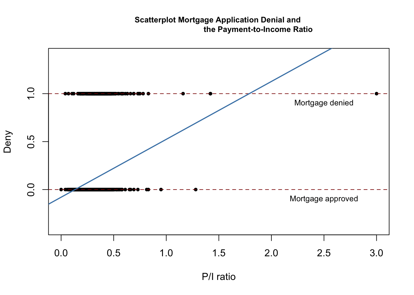
According to the estimated model, a payment-to-income ratio of \(1\) is associated with an expected probability of mortgage application denial of roughly \(50\%\). The model indicates that there is a positive relation between the payment-to-income ratio and the probability of a denied mortgage application so individuals with a high ratio of loan payments to income are more likely to be rejected.
We may use coeftest() to obtain robust standard errors for both coefficient estimates.
# print robust coefficient summary
coeftest(denymod1, vcov. = vcovHC, type = "HC1")
#>
#> t test of coefficients:
#>
#>              Estimate Std. Error t value  Pr(>|t|)
#> (Intercept) -0.079910   0.031967 -2.4998   0.01249 *
#> pirat        0.603535   0.098483  6.1283 1.036e-09 ***
#> ---
#> Signif. codes:  0 '***' 0.001 '**' 0.01 '*' 0.05 '.' 0.1 ' ' 1
The estimated regression line is \[\begin{align} \widehat{deny} = -\underset{(0.032)}{0.080} + \underset{(0.098)}{0.604} P/I \ ratio. \tag{11.2} \end{align}\] The true coefficient on \(P/I \ ratio\) is statistically different from \(0\) at the \(1\%\) level. Its estimate can be interpreted as follows: a 1 percentage point increase in \(P/I \ ratio\) leads to an increase in the probability of a loan denial by \(0.604 \cdot 0.01 = 0.00604 \approx 0.6\%\).
Following the book we augment the simple model (11.1) by an additional regressor \(black\) which equals \(1\) if the applicant is an African American and equals \(0\) otherwise. Such a specification is the baseline for investigating if there is racial discrimination in the mortgage market: if being black has a significant (positive) influence on the probability of a loan denial when we control for factors that allow for an objective assessment of an applicant’s creditworthiness, this is an indicator for discrimination.
# rename the variable 'afam' for consistency
colnames(HMDA)[colnames(HMDA) == "afam"] <- "black"

# estimate the model
denymod2 <- lm(deny ~ pirat + black, data = HMDA)
coeftest(denymod2, vcov. = vcovHC)
#>
#> t test of coefficients:
#>
#>              Estimate Std. Error t value  Pr(>|t|)
#> (Intercept) -0.090514   0.033430 -2.7076  0.006826 **
#> pirat        0.559195   0.103671  5.3939 7.575e-08 ***
#> blackyes     0.177428   0.025055  7.0815 1.871e-12 ***
#> ---
#> Signif. codes:  0 '***' 0.001 '**' 0.01 '*' 0.05 '.' 0.1 ' ' 1
The estimated regression function is \[\begin{align} \widehat{deny} =& \, -\underset{(0.029)}{0.091} + \underset{(0.089)}{0.559} P/I \ ratio + \underset{(0.025)}{0.177} black. \tag{11.3} \end{align}\]
The coefficient on \(black\) is positive and significantly different from zero at the \(0.01\%\) level. The interpretation is that, holding the \(P/I \ ratio\) constant, being black increases the probability of a mortgage application denial by about \(17.7\%\). This finding is compatible with racial discrimination. However, it might be distorted by omitted variable bias so discrimination could be a premature conclusion.