5.5 The Gauss-Markov Theorem
When estimating regression models, we know that the results of the estimation procedure are random. However, when using unbiased estimators, at least on average, we estimate the true parameter. When comparing different unbiased estimators, it is therefore interesting to know which one has the highest precision: being aware that the likelihood of estimating the exact value of the parameter of interest is \(0\) in an empirical application, we want to make sure that the likelihood of obtaining an estimate very close to the true value is as high as possible. This means we want to use the estimator with the lowest variance of all unbiased estimators, provided we care about unbiasedness. The Gauss-Markov theorem states that, in the class of conditionally unbiased linear estimators, the OLS estimator has this property under certain conditions.
Key Concept 5.5
The Gauss-Markov Theorem for \(\hat{\beta}_1\)
Suppose that the assumptions made in Key Concept 4.3 hold and that the errors are homoskedastic. The OLS estimator is the best (in the sense of smallest variance) linear conditionally unbiased estimator (BLUE) in this setting.
Let us have a closer look at what this means:
Estimators of \(\beta_1\) that are linear functions of the \(Y_1, \dots, Y_n\) and that are unbiased conditionally on the regressor \(X_1, \dots, X_n\) can be written as \[ \overset{\sim}{\beta}_1 = \sum_{i=1}^n a_i Y_i. \] where the \(a_i\) are weights that are allowed to depend on the \(X_i\) but not on the \(Y_i\).
We already know that \(\overset{\sim}{\beta}_1\) has a sampling distribution: \(\overset{\sim}{\beta}_1\) is a linear function of the \(Y_i\) which are random variables. If now \[ E(\overset{\sim}{\beta}_1 | X_1, \dots, X_n) = \beta_1, \] \(\overset{\sim}{\beta}_1\) is a linear unbiased estimator of \(\beta_1\), conditionally on the \(X_1, \dots, X_n\).
We may ask if \(\overset{\sim}{\beta}_1\) is also the best estimator in this class, i.e., the most efficient one of all linear conditionally unbiased estimators where “most efficient” means smallest variance. The weights \(a_i\) play an important role here and it turns out that OLS uses just the right weights to have the BLUE property.
Simulation Study: BLUE Estimator
Consider the case of a regression of \(Y_i,\dots,Y_n\) only on a constant. Here, the \(Y_i\) are assumed to be a random sample from a population with mean \(\mu\) and variance \(\sigma^2\). The OLS estimator in this model is simply the sample mean, see Chapter 3.2.
\[\begin{equation} \hat{\beta}_1 = \sum_{i=1}^n \underbrace{\frac{1}{n}}_{=a_i} Y_i. \tag{5.3} \end{equation}\]
Clearly, each observation is weighted by
\[a_i = \frac{1}{n},\]
and we also know that \(\text{Var}(\hat{\beta}_1)=\frac{\sigma^2}{n}\).
We now use R to conduct a simulation study that demonstrates what happens to the variance of (5.3) if different weights \[ w_i = \frac{1 \pm \epsilon}{n} \] are assigned to either half of the sample \(Y_1, \dots, Y_n\) instead of using \(\frac{1}{n}\), the OLS weights.
# set sample size and number of repetitions
n <- 100
reps <- 1e5

# choose epsilon and create a vector of weights as defined above
epsilon <- 0.8
w <- c(rep((1 + epsilon) / n, n / 2),
       rep((1 - epsilon) / n, n / 2) )

# draw a random sample y_1,...,y_n from the standard normal distribution,
# use both estimators 1e5 times and store the result in the vectors 'ols' and
# 'weightedestimator'

ols <- rep(NA, reps)
weightedestimator <- rep(NA, reps)

for (i in 1:reps) {

  y <- rnorm(n)
  ols[i] <- mean(y)
  weightedestimator[i] <- crossprod(w, y)

}

# plot kernel density estimates of the estimators' distributions:

# OLS
plot(density(ols),
     col = "red",
     lwd = 2,
     main = "Density of OLS and Weighted Estimator",
     xlab = "Estimates")

# weighted
lines(density(weightedestimator),
      col = "steelblue",
      lwd = 2)

# add a dashed line at 0 and add a legend to the plot
abline(v = 0, lty = 2)

legend('topright',
       c("OLS", "Weighted"),
       col = c("red", "steelblue"),
       lwd = 2)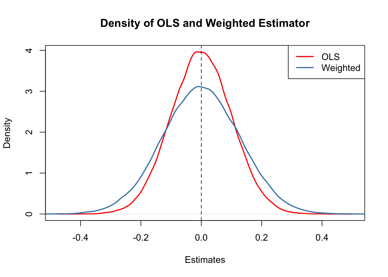
What conclusion can we draw from the result?
- Both estimators seem to be unbiased: the means of their estimated distributions are zero.
- The estimator using weights that deviate from those implied by OLS is less efficient than the OLS estimator: there is higher dispersion when weights are \(w_i = \frac{1 \pm 0.8}{100}\) instead of \(w_i=\frac{1}{100}\) as required by the OLS solution.
Hence, the simulation results support the Gauss-Markov Theorem.