10.2 Panel Data with Two Time Periods: “Before and After” Comparisons
Suppose there are only \(T=2\) time periods \(t=1982,1988\). This allows us to analyze differences in changes of the fatality rate from year 1982 to 1988. We start by considering the population regression model \[FatalityRate_{it} = \beta_0 + \beta_1 BeerTax_{it} + \beta_2 Z_{i} + u_{it}\] where the \(Z_i\) are state specific characteristics that differ between states but are constant over time. For \(t=1982\) and \(t=1988\) we have \[\begin{align*} FatalityRate_{i1982} =&\, \beta_0 + \beta_1 BeerTax_{i1982} + \beta_2 Z_i + u_{i1982}, \\ FatalityRate_{i1988} =&\, \beta_0 + \beta_1 BeerTax_{i1988} + \beta_2 Z_i + u_{i1988}. \end{align*}\]
We can eliminate the \(Z_i\) by regressing the difference in the fatality rate between 1988 and 1982 on the difference in beer tax between those years: \[FatalityRate_{i1988} - FatalityRate_{i1982} = \beta_1 (BeerTax_{i1988} - BeerTax_{i1982}) + u_{i1988} - u_{i1982}.\] This regression model, where the difference in fatality rate between 1988 and 1982 is regressed on the difference in beer tax between those years, yields an estimate for \(\beta_1\) that is robust to a possible bias due to omission of \(Z_i\), as these influences are eliminated from the model. Next we will use R to estimate a regression based on the differenced data and to plot the estimated regression function.
# compute the differences
diff_fatal_rate <- Fatalities1988$fatal_rate - Fatalities1982$fatal_rate
diff_beertax <- Fatalities1988$beertax - Fatalities1982$beertax

# estimate a regression using differenced data
fatal_diff_mod <- lm(diff_fatal_rate ~ diff_beertax)

coeftest(fatal_diff_mod, vcov = vcovHC, type = "HC1")
#>
#> t test of coefficients:
#>
#>               Estimate Std. Error t value Pr(>|t|)
#> (Intercept)  -0.072037   0.065355 -1.1022 0.276091
#> diff_beertax -1.040973   0.355006 -2.9323 0.005229 **
#> ---
#> Signif. codes:  0 '***' 0.001 '**' 0.01 '*' 0.05 '.' 0.1 ' ' 1
Including the intercept allows for a change in the mean fatality rate in the time between 1982 and 1988 in the absence of a change in the beer tax.
We obtain the OLS estimated regression function \[\widehat{FatalityRate_{i1988} - FatalityRate_{i1982}} = -\underset{(0.065)}{0.072} -\underset{(0.36)}{1.04} \times (BeerTax_{i1988}-BeerTax_{i1982}).\]
# plot the differenced data
plot(x = as.double(diff_beertax),
     y = as.double(diff_fatal_rate),
     xlab = "Change in beer tax (in 1988 dollars)",
     ylab = "Change in fatality rate (fatalities per 10000)",
     main = "Changes in Traffic Fatality Rates and Beer Taxes in 1982-1988",
     cex.main=1,
     xlim = c(-0.6, 0.6),
     ylim = c(-1.5, 1),
     pch = 20,
     col = "steelblue")

# add the regression line to plot
abline(fatal_diff_mod, lwd = 1.5,col="darkred")
#add legend
legend("topright",lty=1,col="darkred","Estimated Regression Line")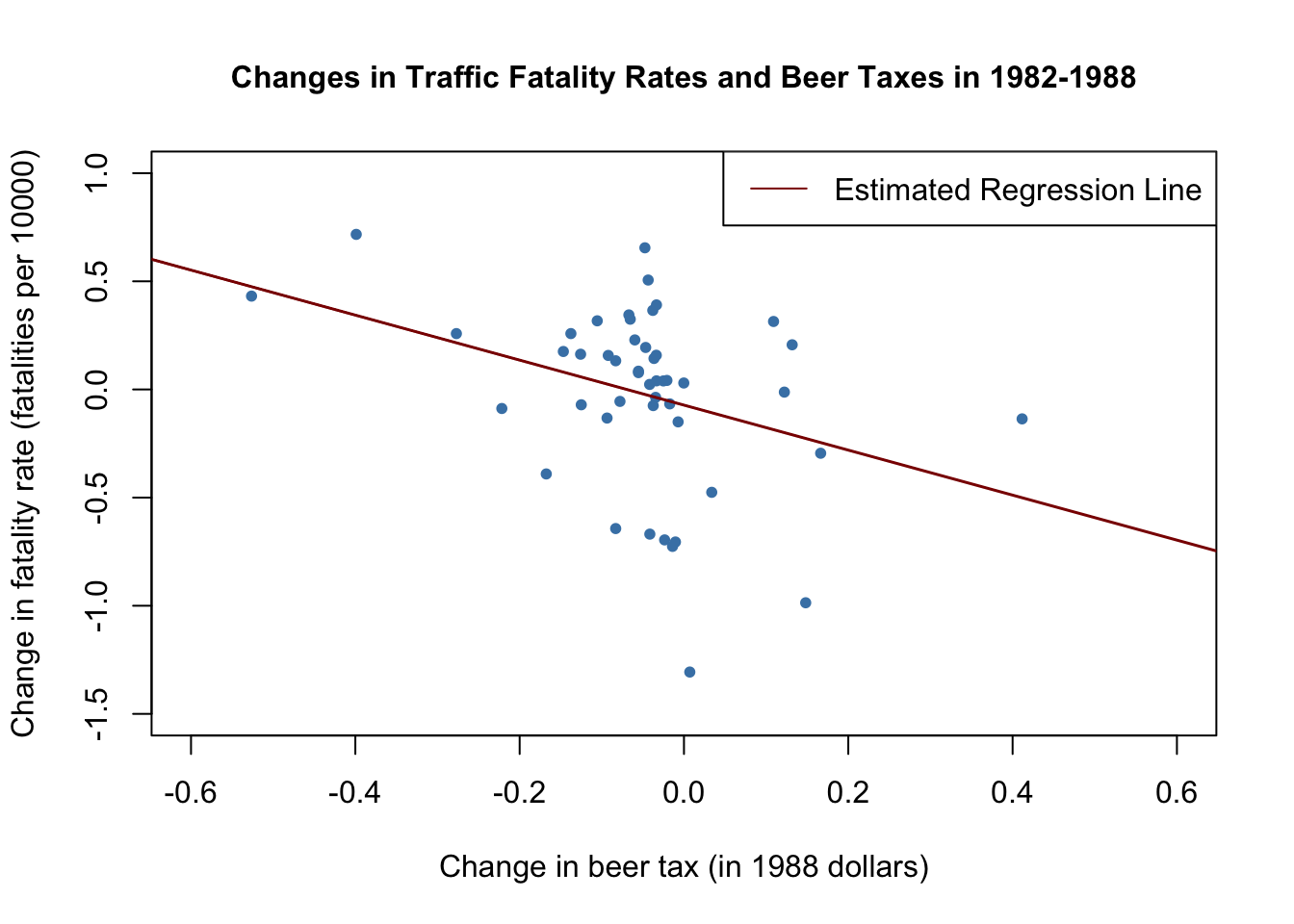
The estimated coefficient on beer tax is now negative and significantly different from zero at \(5\%\). Its interpretation is that raising the beer tax by \(\$1\) causes traffic fatalities to decrease by \(1.04\) per \(10000\) people. This is rather large as the average fatality rate is approximately \(2\) persons per \(10000\) people.
# compute mean fatality rate over all states for all time periods
mean(Fatalities$fatal_rate)
#> [1] 2.040444
Once more this outcome is likely to be a consequence of omitting factors in the single-year regression that influence the fatality rate and are correlated with the beer tax and change over time. The message is that we need to be more careful and control for such factors before drawing conclusions about the effect of a raise in beer taxes.
The approach presented in this section discards information for years \(1983\) to \(1987\). The fixed effects method that allows us to use data for more than \(T = 2\) time periods and enables us to add control variables to the analysis.