7.6 Analysis of the Test Score Data Set
Chapter 6 and some of the previous sections have stressed that it is important to include control variables in regression models if it is plausible that there are omitted factors. In our example of test scores, we want to estimate the causal effect of a change in the student-teacher ratio on test scores. We now provide an example of how to use multiple regression in order to alleviate omitted variable bias and demonstrate how to report this results using R.
So far we have considered two variables that control for unobservable student characteristics which correlate with the student-teacher ratio and are assumed to have an impact on test scores:
\(English\), the percentage of English learning students.
\(lunch\), the share of students that qualify for a subsidized or even a free lunch at school.
Another new variable provided with CASchools is calworks, the percentage of students that qualify for the CalWorks income assistance program. Students eligible for CalWorks live in families with a total income below the threshold for the subsidized lunch program so both variables are indicators for the share of economically disadvantaged children. Both indicators are highly correlated.
# estimate the correlation between 'calworks' and 'lunch'
cor(CASchools$calworks, CASchools$lunch)
#> [1] 0.7394218
There is no unambiguous way to proceed when deciding which variable to use. In any case it may not be a good idea to use both variables as regressors in view of collinearity. Therefore, we also consider alternative model specifications.
For a start, we plot student characteristics against test scores.
# set up arrangement of plots
m <- rbind(c(1, 2), c(3, 0))
graphics::layout(mat = m)

# scatterplots
plot(score ~ english,
     data = CASchools,
     col = "steelblue",
     pch = 20,
     xlim = c(0, 100),
     cex.main = 0.7,
     xlab="English",
     ylab="Score",
     main = "Percentage of English language learners")

plot(score ~ lunch,
     data = CASchools,
     col = "steelblue",
     pch = 20,
     cex.main = 0.7,
     xlab="Lunch",
     ylab="Score",
     main = "Percentage qualifying for reduced price lunch")

plot(score ~ calworks,
     data = CASchools,
     col = "steelblue",
     pch = 20,
     xlim = c(0, 100),
     cex.main = 0.7,
     xlab="CalWorks",
     ylab="Score",
     main = "Percentage qualifying for income assistance")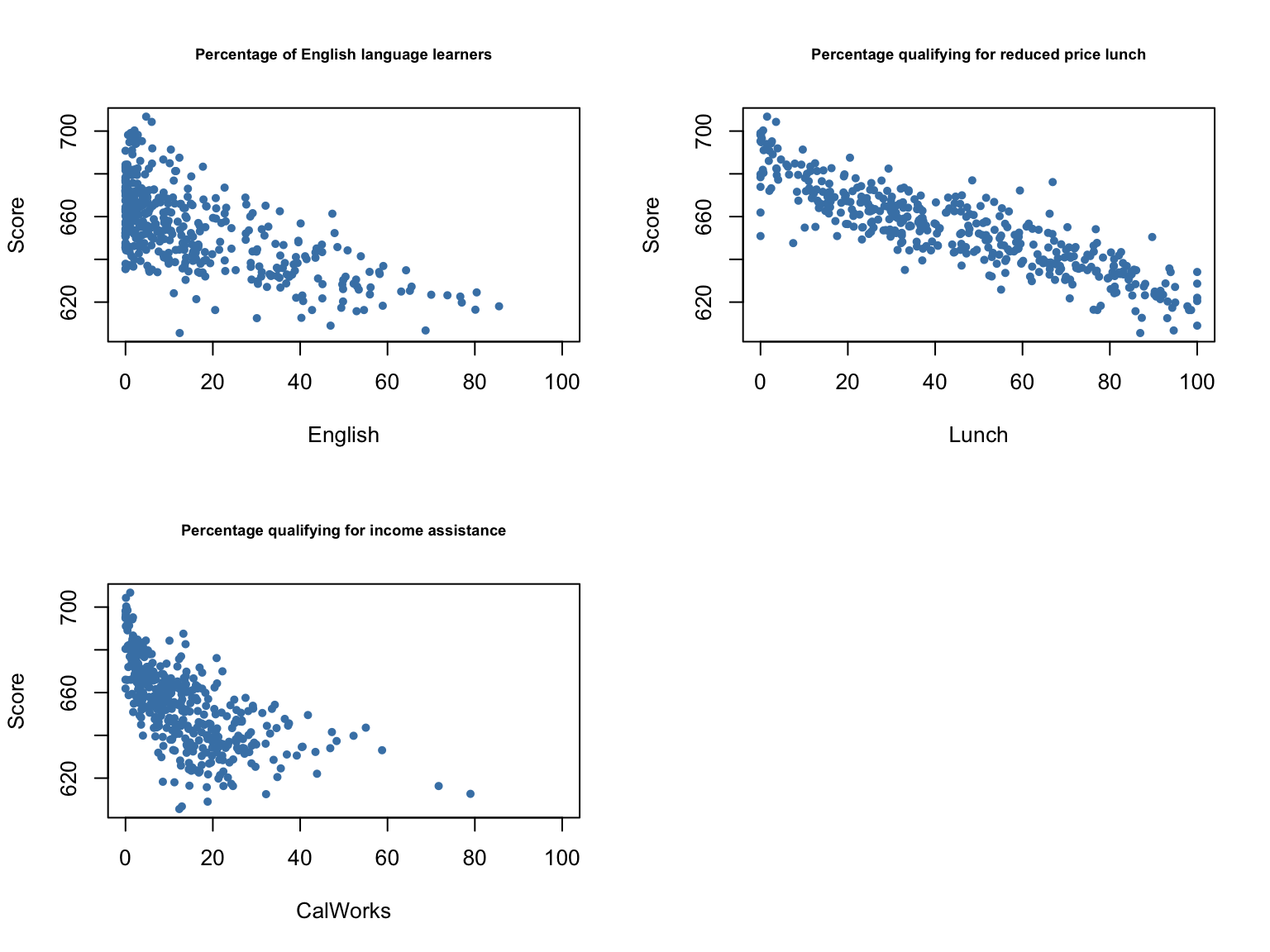
We divide the plotting area up using layout(). The matrix m specifies the location of the plots, see ?layout.
We see that all relationships are negative. Here are the correlation coefficients.
# estimate correlation between student characteristics and test scores
cor(CASchools$score, CASchools$english)
#> [1] -0.6441238
cor(CASchools$score, CASchools$lunch)
#> [1] -0.868772
cor(CASchools$score, CASchools$calworks)
#> [1] -0.6268533
We shall consider five different model equations:
\[\begin{align*} (I) \quad TestScore=& \, \beta_0 + \beta_1 \times STR + u, \\ (II) \quad TestScore=& \, \beta_0 + \beta_1 \times STR + \beta_2 \times english + u, \\ (III) \quad TestScore=& \, \beta_0 + \beta_1 \times STR + \beta_2 \times english + \beta_3 \times lunch + u, \\ (IV) \quad TestScore=& \, \beta_0 + \beta_1 \times STR + \beta_2 \times english + \beta_4 \times calworks + u, \\ (V) \quad TestScore=& \, \beta_0 + \beta_1 \times STR + \beta_2 \times english + \beta_3 \times lunch + \beta_4 \times calworks + u. \end{align*}\]
The best way to communicate regression results is in a table. The stargazer package is very convenient for this purpose. It provides a function that generates professionally looking HTML and LaTeX tables that satisfy scientific standards. One simply has to provide one or multiple object(s) of class lm. The rest is done by the function stargazer().
# load the stargazer library
library(stargazer)

# estimate different model specifications
spec1 <- lm(score ~ STR, data = CASchools)
spec2 <- lm(score ~ STR + english, data = CASchools)
spec3 <- lm(score ~ STR + english + lunch, data = CASchools)
spec4 <- lm(score ~ STR + english + calworks, data = CASchools)
spec5 <- lm(score ~ STR + english + lunch + calworks, data = CASchools)

# gather robust standard errors in a list
rob_se <- list(sqrt(diag(vcovHC(spec1, type = "HC1"))),
               sqrt(diag(vcovHC(spec2, type = "HC1"))),
               sqrt(diag(vcovHC(spec3, type = "HC1"))),
               sqrt(diag(vcovHC(spec4, type = "HC1"))),
               sqrt(diag(vcovHC(spec5, type = "HC1"))))

# generate a LaTeX table using stargazer
stargazer(spec1, spec2, spec3, spec4, spec5,
          se = rob_se,
          digits = 3,
          header = F,
column.labels = c("(I)", "(II)", "(III)", "(IV)", "(V)"))| Dependent Variable: Test Score | |||||
| score | |||||
| (I) | (II) | (III) | (IV) | (V) | |
| spec1 | spec2 | spec3 | spec4 | spec5 | |
| STR | -2.280*** | -1.101** | -0.998*** | -1.308*** | -1.014*** |
| (0.519) | (0.433) | (0.270) | (0.339) | (0.269) | |
| english | -0.650*** | -0.122*** | -0.488*** | -0.130*** | |
| (0.031) | (0.033) | (0.030) | (0.036) | ||
| lunch | -0.547*** | -0.529*** | |||
| (0.024) | (0.038) | ||||
| calworks | -0.790*** | -0.048 | |||
| (0.068) | (0.059) | ||||
| Constant | 698.933*** | 686.032*** | 700.150*** | 697.999*** | 700.392*** |
| (10.364) | (8.728) | (5.568) | (6.920) | (5.537) | |
| Observations | 420 | 420 | 420 | 420 | 420 |
| R2 | 0.051 | 0.426 | 0.775 | 0.629 | 0.775 |
| Adjusted R2 | 0.049 | 0.424 | 0.773 | 0.626 | 0.773 |
| Residual Std. Error | 18.581 (df = 418) | 14.464 (df = 417) | 9.080 (df = 416) | 11.654 (df = 416) | 9.084 (df = 415) |
| F Statistic | 22.575*** (df = 1; 418) | 155.014*** (df = 2; 417) | 476.306*** (df = 3; 416) | 234.638*** (df = 3; 416) | 357.054*** (df = 4; 415) |
| Note: | *p<0.1; **p<0.05; ***p<0.01 | ||||
Table 7.1: Regressions of Test Scores on the Student-Teacher Ratio and Control Variables
Table 7.1 states that \(score\) is the dependent variable and that we consider five models. We see that the columns of Table 7.1 contain most of the information provided by coeftest() and summary() for the regression models under consideration: the coefficients estimates equipped with significance codes (the asterisks) and standard errors in parentheses below. Although there are no \(t\)-statistics, it is straightforward for the reader to compute them simply by dividing a coefficient estimate by the corresponding standard error. The bottom of the table reports summary statistics for each model and a legend. For an in-depth discussion of the tabular presentation of regression results, see Chapter 7.6 of the book.
What can we conclude from the model comparison?
We see that adding control variables roughly halves the coefficient on STR. Also, the estimate is not sensitive to the set of control variables used. The conclusion is that decreasing the student-teacher ratio ceteris paribus by one unit leads to an estimated average increase in test scores of about \(1\) point.
Adding student characteristics as controls increases \(R^2\) and \(\bar{R}^2\) from \(0.049\) (spec1) up to \(0.773\) (spec3 and spec5), so we can consider these variables as suitable predictors for test scores. Moreover, the estimated coefficients on all control variables are consistent with the impressions gained from Figure 7.2 of the book.
We see that the control variables are not statistically significant in all models. For example in spec5, the coefficient on \(calworks\) is not significantly different from zero at \(5\%\) since \(\lvert-0.048/0.059\rvert=0.81 < 1.64\). We also observe that the effect on the estimate (and its standard error) of the coefficient on \(size\) of adding \(calworks\) to the base specification spec3 is negligible. We can therefore consider calworks as a superfluous control variable, given the inclusion of lunch in this model.