16.3 Cointegration
Key Concept
16.5
Cointegration
When \(X_t\) and \(Y_t\) are \(I(1)\) and if there is a \(\theta\) such that \(Y_t - \theta X_t\) is \(I(0)\), \(X_t\) and \(Y_t\) are cointegrated. Put differently, cointegration of \(X_t\) and \(Y_t\) means that \(X_t\) and \(Y_t\) have the same or a common stochastic trend and that this trend can be eliminated by taking a specific difference of the series such that the resulting series is stationary.
R functions for cointegration analysis are implemented in the package urca.
As an example, reconsider the relation between short-term and long-term interest rates in the example of U.S. 3-month treasury bills, U.S. 10-years treasury bonds and the spread in their interest rates which have been introduced in Chapter 14.4. The next code chunk shows how to reproduce Figure 16.2 of the book.
# reproduce Figure 16.2 of the book

# plot both interest series
plot(merge(as.zoo(TB3MS), as.zoo(TB10YS)),
     plot.type = "single",
     lty = c(2, 1),
     lwd = 2,
     xlab = "Date",
     ylab = "Percent per annum",
     ylim = c(-5, 17),
     main = "Interest Rates")

# add the term spread series
lines(as.zoo(TSpread),
     col = "steelblue",
     lwd = 2,
     xlab = "Date",
     ylab = "Percent per annum",
     main = "Term Spread")

# shade the term spread
polygon(c(time(TB3MS), rev(time(TB3MS))),
        c(TB10YS, rev(TB3MS)),
        col = alpha("steelblue", alpha = 0.3),
        border = NA)

# add horizontal line at 0
abline(0, 0)

# add a legend
legend("topright",
       legend = c("TB3MS", "TB10YS", "Term Spread"),
       col = c("black", "black", "steelblue"),
       lwd = c(2, 2, 2),
       lty = c(2, 1, 1))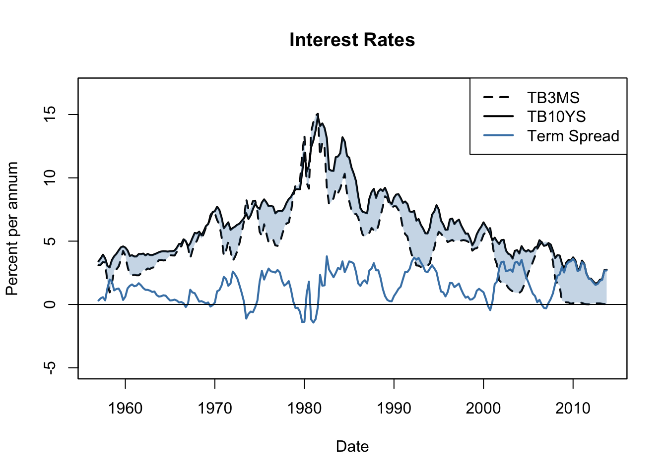
The plot suggests that long-term and short-term interest rates are cointegrated: both interest series seem to have the same long-run behavior. They share a common stochastic trend. The term spread, which is obtained by taking the difference between long-term and short-term interest rates, seems to be stationary. In fact, the expectations theory of the term structure suggests the cointegrating coefficient \(\theta\) to be 1. This is consistent with the visual result.
Testing for Cointegration
Following Key Concept 16.5, it seems natural to construct a test for cointegration of two series in the following manner: if two series \(X_t\) and \(Y_t\) are cointegrated, the series obtained by taking the difference \(Y_t - \theta X_t\) must be stationary. If the series are not cointegrated, \(Y_t - \theta X_t\) is nonstationary. This is an assumption that can be tested using a unit root test. We have to distinguish between two cases:
\(\theta\) is known.
Knowledge of \(\theta\) enables us to compute differences \(z_t = Y_t - \theta X_t\) so that Dickey-Fuller and DF-GLS unit root tests can be applied to \(z_t\). For these tests, the critical values are the critical values of the ADF or DF-GLS test.
\(\theta\) is unknown.
If \(\theta\) is unknown, it must be estimated before the unit root test can be applied. This is done by estimating the regression \[Y_t = \alpha + \theta X_t + z_t\] using OLS (this is refered to as the first-stage regression). Then, a Dickey-Fuller test is used for testing the hypothesis that \(z_t\) is a nonstationary series. This is known as the Engle-Granger Augmented Dickey-Fuller test for cointegration (or EG-ADF test) after Engle and Granger (1987). The critical values for this test are special as the associated null distribution is nonnormal and depends on the number of \(I(1)\) variables used as regressors in the first stage regression. You may look them up in Table 16.2 of the book. When there are only two presumably cointegrated variables (and thus a single \(I(1)\) variable is used in the first stage OLS regression) the critical values for the levels \(10\%\), \(5\%\) and \(1\%\) are \(-3.12\), \(-3.41\) and \(-3.96\).
Application to Interest Rates
As has been mentioned above, the theory of the term structure suggests that long-term and short-term interest rates are cointegrated with a cointegration coefficient of \(\theta = 1\). In the previous section we have seen that there is visual evidence for this conjecture since the spread of 10-year and 3-month interest rates looks stationary.
We continue by using formal tests (the ADF and the DF-GLS test) to see whether the individual interest rate series are integrated and if their difference is stationary (for now, we assume that \(\theta = 1\) is known). Both is conveniently done by using the functions ur.df() for computation of the ADF test and ur.ers for conducting the DF-GLS test. Following the book we use data from 1962:Q1 to 2012:Q4 and employ models that include a drift term. We set the maximum lag order to \(6\) and use the \(AIC\) for selection of the optimal lag length.
# test for nonstationarity of 3-month treasury bills using ADF test
ur.df(window(TB3MS, c(1962, 1), c(2012, 4)),
      lags = 6,
      selectlags = "AIC",
      type = "drift")
#>
#> ###############################################################
#> # Augmented Dickey-Fuller Test Unit Root / Cointegration Test #
#> ###############################################################
#>
#> The value of the test statistic is: -2.1004 2.2385

# test for nonstationarity of 10-years treasury bonds using ADF test
ur.df(window(TB10YS, c(1962, 1), c(2012, 4)),
      lags = 6,
      selectlags = "AIC",
      type = "drift")
#>
#> ###############################################################
#> # Augmented Dickey-Fuller Test Unit Root / Cointegration Test #
#> ###############################################################
#>
#> The value of the test statistic is: -1.0079 0.5501

# test for nonstationarity of 3-month treasury bills using DF-GLS test
ur.ers(window(TB3MS, c(1962, 1), c(2012, 4)),
       model = "constant",
       lag.max = 6)
#>
#> ###############################################################
#> # Elliot, Rothenberg and Stock Unit Root / Cointegration Test #
#> ###############################################################
#>
#> The value of the test statistic is: -1.8042

# test for nonstationarity of 10-years treasury bonds using DF-GLS test
ur.ers(window(TB10YS, c(1962, 1), c(2012, 4)),
       model = "constant",
       lag.max = 6)
#>
#> ###############################################################
#> # Elliot, Rothenberg and Stock Unit Root / Cointegration Test #
#> ###############################################################
#>
#> The value of the test statistic is: -0.942
The corresponding \(10\%\) critical value for both tests is \(-2.57\) so we cannot reject the null hypotheses of nonstationary for either series, even at the \(10\%\) level of significance.12 We conclude that it is plausible to model both interest rate series as \(I(1)\).
Next, we apply the ADF and the DF-GLS test to test for nonstationarity of the term spread series, which means we test for non-cointegration of long- and short-term interest rates.
# test if term spread is stationary (cointegration of interest rates) using ADF
ur.df(window(TB10YS, c(1962, 1), c(2012, 4)) - window(TB3MS, c(1962, 1), c(2012 ,4)),
      lags = 6,
      selectlags = "AIC",
      type = "drift")
#>
#> ###############################################################
#> # Augmented Dickey-Fuller Test Unit Root / Cointegration Test #
#> ###############################################################
#>
#> The value of the test statistic is: -3.9308 7.7362

# test if term spread is stationary (cointegration of interest rates) using DF-GLS
ur.ers(window(TB10YS, c(1962, 1), c(2012, 4)) - window(TB3MS, c(1962, 1),c(2012, 4)),
       model = "constant",
       lag.max = 6)
#>
#> ###############################################################
#> # Elliot, Rothenberg and Stock Unit Root / Cointegration Test #
#> ###############################################################
#>
#> The value of the test statistic is: -3.8576
Table 16.1 summarizes the results.
| Series | ADF Test Statistic | DF-GLS Test Statistic |
|---|---|---|
| TB3MS | \(-2.10\) | \(-1.80\) |
| TB10YS | \(-1.01\) | \(-0.94\) |
| TB10YS - TB3MS | \(-3.93\) | \(-3.86\) |
Both tests reject the hypothesis of nonstationarity of the term spread series at the \(1\%\) level of significance, which is strong evidence in favor of the hypothesis that the term spread is stationary, implying cointegration of long- and short-term interest rates.
Since theory suggests that \(\theta=1\), there is no need to estimate \(\theta\) so it is not necessary to use the EG-ADF test which allows \(\theta\) to be unknown. However, since it is instructive to do so, we follow the book and compute this test statistic. The first-stage OLS regression is \[TB10YS_t = \beta_0 + \beta_1 TB3MS_t + z_t.\]
# estimate first-stage regression of EG-ADF test
FS_EGADF <- dynlm(window(TB10YS, c(1962, 1), c(2012, 4)) ~ window(TB3MS, c(1962, 1),
                                                                  c(2012, 4)))
FS_EGADF
#>
#> Time series regression with "ts" data:
#> Start = 1962(1), End = 2012(4)
#>
#> Call:
#> dynlm(formula = window(TB10YS, c(1962, 1), c(2012, 4)) ~ window(TB3MS,
#>     c(1962, 1), c(2012, 4)))
#>
#> Coefficients:
#>                           (Intercept)  window(TB3MS, c(1962, 1), c(2012, 4))
#>                                2.4642                                 0.8147
Thus we have \[\begin{align*} \widehat{TB10YS}_t = 2.46 + 0.81 \cdot TB3MS_t, \end{align*}\] where \(\widehat{\theta} = 0.81\). Next, we take the residual series \(\{\widehat{z_t}\}\) and compute the ADF test statistic.
# compute the residuals
z_hat <- resid(FS_EGADF)

# compute the ADF test statistic
ur.df(z_hat, lags = 6, type = "none", selectlags = "AIC")
#>
#> ###############################################################
#> # Augmented Dickey-Fuller Test Unit Root / Cointegration Test #
#> ###############################################################
#>
#> The value of the test statistic is: -3.1935
The test statistic is \(-3.19\) which is smaller than the \(10\%\) critical value but larger than the \(5\%\) critical value (see Table 16.2 of the book). Thus, the null hypothesis of no cointegration can be rejected at the \(10\%\) level but not at the \(5\%\) level. This indicates lower power of the EG-ADF test due to the estimation of \(\theta\): when \(\theta=1\) is the correct value, we expect the power of the ADF test for a unit root in the residuals series \(\widehat{z} = TB10YS - TB3MS\) to be higher than when some estimate \(\widehat{\theta}\) is used.
A Vector Error Correction Model for \(TB10YS_t\) and \(TB3MS\)
If two \(I(1)\) time series \(X_t\) and \(Y_t\) are cointegrated, their differences are stationary and can be modeled in a VAR which is augmented by the regressor \(Y_{t-1} - \theta X_{t-1}\). This is called a vector error correction model (VECM) and \(Y_{t} - \theta X_{t}\) is called the error correction term. Lagged values of the error correction term are useful for predicting \(\Delta X_t\) and/or \(\Delta Y_t\).
A VECM can be used to model the two interest rates considered in the previous sections. Following the book we specify the VECM to include two lags of both series as regressors and choose \(\theta = 1\), as theory suggests (see above).
TB10YS <- window(TB10YS, c(1962, 1), c(2012 ,4))
TB3MS <- window(TB3MS, c(1962, 1), c(2012, 4))

# set up error correction term
VECM_ECT <- TB10YS - TB3MS

# estimate both equations of the VECM using 'dynlm()'
VECM_EQ1 <- dynlm(d(TB10YS) ~ L(d(TB3MS), 1:2) + L(d(TB10YS), 1:2) + L(VECM_ECT))
VECM_EQ2 <- dynlm(d(TB3MS) ~ L(d(TB3MS), 1:2) + L(d(TB10YS), 1:2) + L(VECM_ECT))

# rename regressors for better readability
names(VECM_EQ1$coefficients) <- c("Intercept", "D_TB3MS_l1", "D_TB3MS_l2",
                                  "D_TB10YS_l1", "D_TB10YS_l2", "ect_l1")
names(VECM_EQ2$coefficients) <- names(VECM_EQ1$coefficients)

# coefficient summaries using HAC standard errors
coeftest(VECM_EQ1, vcov. = NeweyWest(VECM_EQ1, prewhite = F, adjust = T))
#>
#> t test of coefficients:
#>
#>               Estimate Std. Error t value Pr(>|t|)
#> Intercept    0.1227089  0.0551419  2.2253 0.027205 *
#> D_TB3MS_l1  -0.0016601  0.0727060 -0.0228 0.981807
#> D_TB3MS_l2  -0.0680845  0.0435059 -1.5649 0.119216
#> D_TB10YS_l1  0.2264878  0.0957071  2.3665 0.018939 *
#> D_TB10YS_l2 -0.0734486  0.0703476 -1.0441 0.297740
#> ect_l1      -0.0878871  0.0285644 -3.0768 0.002393 **
#> ---
#> Signif. codes:  0 '***' 0.001 '**' 0.01 '*' 0.05 '.' 0.1 ' ' 1
coeftest(VECM_EQ2, vcov. = NeweyWest(VECM_EQ2, prewhite = F, adjust = T))
#>
#> t test of coefficients:
#>
#>              Estimate Std. Error t value Pr(>|t|)
#> Intercept   -0.060746   0.107937 -0.5628  0.57422
#> D_TB3MS_l1   0.240003   0.111611  2.1504  0.03276 *
#> D_TB3MS_l2  -0.155883   0.153845 -1.0132  0.31220
#> D_TB10YS_l1  0.113740   0.125571  0.9058  0.36617
#> D_TB10YS_l2 -0.147519   0.112630 -1.3098  0.19182
#> ect_l1       0.031506   0.050519  0.6236  0.53359
#> ---
#> Signif. codes:  0 '***' 0.001 '**' 0.01 '*' 0.05 '.' 0.1 ' ' 1
Thus the two estimated equations of the VECM are \[\begin{align*} \widehat{\Delta TB3MS}_t =& \, -\underset{(0.11)}{0.06} + \underset{(0.11)}{0.24} \Delta TB3MS_{t-1} -\underset{(0.15)}{0.16} \Delta TB3MS_{t-2} \\ &+ \underset{(0.13)}{0.11} \Delta TB10YS_{t-1} -\underset{(0.11)}{0.15} \Delta TB10YS_{t-2} + \underset{(0.05)}{0.03} ECT_{t-1}, and, \\ \widehat{\Delta TB10YS}_t =& \, \underset{(0.06)}{0.12} -\underset{(0.07)}{0.00} \Delta TB3MS_{t-1} -\underset{(0.04)}{0.07} \Delta TB3MS_{t-2} \\ &+ \underset{(0.10)}{0.23} \Delta TB10YS_{t-1} -\underset{(0.07)}{0.07} \Delta TB10YS_{t-2} -\underset{(0.03)}{0.09} ECT_{t-1}. \end{align*}\]
The output produced by coeftest() shows that there is little evidence that lagged values of the differenced interest series are useful for prediction. This finding is more pronounced for the equation of the differenced series of the 3-month treasury bill rate, where the error correction term (the lagged term spread) is not significantly different from zero at any common level of significance. However, for the differenced 10-years treasury bonds rate the error correction term is statistically significant at \(1\%\) with an estimate of \(-0.09\). This can be interpreted as follows: although both interest rates are nonstationary, their conintegrating relationship allows to predict the change in the 10-years treasury bonds rate using the VECM. In particular, the negative estimate of the coefficient on the error correction term indicates that there will be a negative change in the next period’s 10-years treasury bonds rate when the 10-years treasury bonds rate is unusually high relative to the 3-month treasury bill rate in the current period.
References
Note: ur.df() reports two test statistics when there is a drift in the ADF regression. The first of which (the one we are interested in here) is the \(t\)-statistic for the test that the coefficient on the first lag of the series is 0. The second one is the \(t\)-statistic for the hypothesis test that the drift term equals \(0\).↩︎