15.5 Estimation of Dynamic Causal Effects with Strictly Exogeneous Regressors
In general, the errors in a distributed lag model are correlated which necessitates usage of HAC standard errors for valid inference. If, however, the assumption of exogeneity (the first assumption stated in Key Concept 15.1) is replaced by strict exogeneity, that is, \[E(u_t\vert \dots, X_{t+1}, X_{t}, X_{t-1}, \dots) = 0,\] more efficient approaches than OLS estimation of the coefficients become available. For a general distributed lag model with \(r\) lags and AR(\(p\)) errors, these approaches are summarized in Key Concept 15.4.
Key Concept 15.4
Estimation of Dynamic Multipliers Under Strict Exogeneity
Consider the general distributed lag model with \(r\) lags and errors following an AR(\(p\)) process, \[\begin{align} Y_t =& \, \beta_0 + \beta_1 X_t + \beta_2 X_{t-1} + \dots + \beta_{r+1} X_{t-r} + u_t \tag{15.7} \\ u_t =& \, \phi_1 u_{t-1} + \phi u_{t-2} + \dots + \phi_p u_{t-p} + \overset{\sim}{u}_t. \tag{15.8} \end{align}\] Under strict exogeneity of \(X_t\), one may rewrite the above model in the ADL specification \[\begin{align*} Y_t =& \, \alpha_0 + \phi_1 Y_{t-1} + \phi_2 Y_{t-2} + \dots + \phi_p Y_{t-p} \\ &+ \, \delta_0 X_t + \delta_1 X_{t-1} + \dots + \delta_q X_{t-q} + \overset{\sim}{u}_t \end{align*}\] where \(q=r+p\) and compute estimates of the dynamic multipliers \(\beta_1, \beta_2, \dots, \beta_{r+1}\) using OLS estimates of \(\phi_1, \phi_2, \dots, \phi_p, \delta_0, \delta_1, \dots, \delta_q\).
An alternative is to estimate the dynamic multipliers using feasible GLS, that is to apply the OLS estimator to a quasi-difference specification of (15.7). Under strict exogeneity, the feasible GLS approach is the BLUE estimator for the dynamic multipliers in large samples.
On the one hand, as demonstrated in Chapter 15.5 of the book, OLS estimation of the ADL representation can be beneficial for estimation of the dynamic multipliers in large distributed lag models because it allows for a more parsimonious model that may be a good approximation to the large model. On the other hand, the GLS approach is more efficient than the ADL estimator if the sample size is large.We shortly review how the different representations of a small distributed lag model can be obtained and show how this specification can be estimated by OLS and GLS using R.
The model is \[\begin{align} Y_t = \beta_0 + \beta_1 X_t + \beta_2 X_{t-1} + u_t, \tag{15.9} \end{align}\] so a change in \(X\) is modeled to effect \(Y\) contemporaneously (\(\beta_1\)) and in the next period (\(\beta_2\)). The error term \(u_t\) is assumed to follow an AR(\(1\)) process,\[u_t = \phi_1 u_{t-1} + \overset{\sim}{u_t},\] where \(\overset{\sim}{u_t}\) is serially uncorrelated.
One can show that the ADL representation of this model is \[\begin{align} Y_t = \alpha_0 + \phi_1 Y_{t-1} + \delta_0 X_t + \delta_1 X_{t-1} + \delta_2 X_{t-2} + \overset{\sim}{u}_t, \tag{15.10} \end{align}\] with the restrictions \[\begin{align*} \beta_1 =& \, \delta_0, \\ \beta_2 =& \, \delta_1 + \phi_1 \delta_0, \end{align*}\] see p. 657 of the book.
Quasi-Differences
Another way of writing the ADL(\(1\),\(2\)) representation (15.10) is the quasi-difference model \[\begin{align} \overset{\sim}{Y}_t = \alpha_0 + \beta_1 \overset{\sim}{X}_t + \beta_2 \overset{\sim}{X}_{t-1} + \overset{\sim}{u}_t, \tag{15.11} \end{align}\] where \(\overset{\sim}{Y}_t = Y_t - \phi_1 Y_{t-1}\) and \(\overset{\sim}{X}_t = X_t - \phi_1 X_{t-1}\). Notice that the error term \(\overset{\sim}{u}_t\) is uncorrelated in both models and, as shown in Chapter 15.5 of the book, \[E(u_t\vert X_{t+1}, X_t, X_{t-1}, \dots) = 0,\] which is implied by the assumption of strict exogeneity.
We continue by simulating a time series of \(500\) observations using the model (15.9) with \(\beta_1 = 0.1\), \(\beta_2 = 0.25\), \(\phi = 0.5\) and \(\overset{\sim}{u}_t \sim \mathcal{N}(0,1)\) and estimate the different representations, starting with the distributed lag model (15.9).
# set seed for reproducibility
set.seed(1)

# simulate a time series with serially correlated errors
obs <- 501
eps <- arima.sim(n = obs-1 , model = list(ar = 0.5))
X <- arima.sim(n = obs, model = list(ar = 0.25))
Y <- 0.1 * X[-1] + 0.25 * X[-obs] + eps
X <- ts(X[-1])

# estimate the distributed lag model
dlm <- dynlm(Y ~ X + L(X))
Let us check that the residuals of this model exhibit autocorrelation using acf().
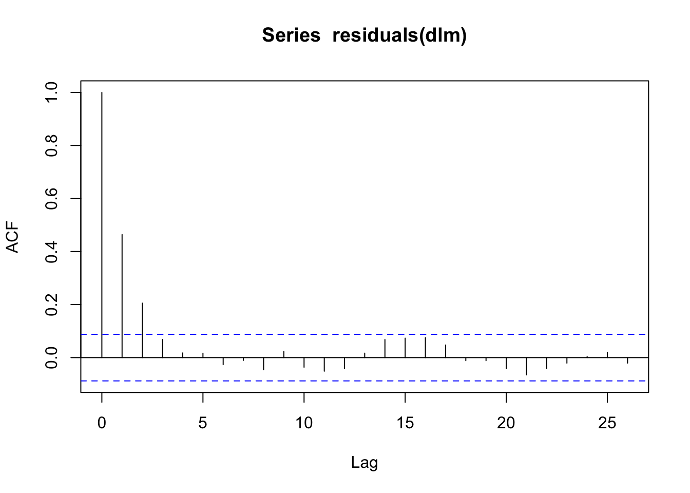
In particular, the pattern reveals that the residuals follow an autoregressive process, as the sample autocorrelation function decays quickly for the first few lags and is probably zero for higher lag orders. In any case, HAC standard errors should be used.
# coefficient summary using the Newey-West SE estimates
coeftest(dlm, vcov = NeweyWest, prewhite = F, adjust = T)
#>
#> t test of coefficients:
#>
#>             Estimate Std. Error t value  Pr(>|t|)
#> (Intercept) 0.038340   0.073411  0.5223  0.601717
#> X           0.123661   0.046710  2.6474  0.008368 **
#> L(X)        0.247406   0.046377  5.3347 1.458e-07 ***
#> ---
#> Signif. codes:  0 '***' 0.001 '**' 0.01 '*' 0.05 '.' 0.1 ' ' 1
OLS Estimation of the ADL Model
Next, we estimate the ADL(\(1\),\(2\)) model (15.10) using OLS. The errors are uncorrelated in this representation of the model. This statement is supported by a plot of the sample autocorrelation function of the residual series.
# estimate the ADL(2,1) representation of the distributed lag model
adl21_dynamic <- dynlm(Y ~ L(Y) + X + L(X, 1:2))

# plot the sample autocorrelaltions of residuals
acf(adl21_dynamic$residuals)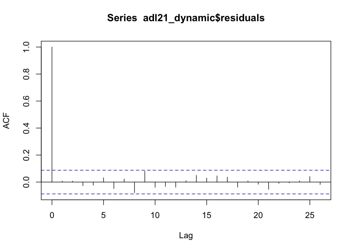
The estimated coefficients of adl21_dynamic$coefficients are not the dynamic multipliers we are interested in, but instead can be computed according to the restrictions in (15.10), where the true coefficients are replaced by the OLS estimates.
GLS Estimation
Strict exogeneity allows for OLS estimation of the quasi-difference model (15.11). The idea of applying the OLS estimator to a model where the variables are linearly transformed, such that the model errors are uncorrelated and homoskedastic, is called generalized least squares (GLS).
The OLS estimator in (15.11) is called the infeasible GLS estimator because \(\overset{\sim}{Y}\) and \(\overset{\sim}{X}\) cannot be computed without knowing \(\phi_1\), the autoregressive coefficient in the error AR(\(1\)) model, which is generally unknown in practice.
Assume we knew that \(\phi = 0.5\). We then may obtain the infeasible GLS estimates of the dynamic multipliers in (15.9) by applying OLS to the transformed data.
# GLS: estimate quasi-differenced specification by OLS
iGLS_dynamic <- dynlm(I(Y- 0.5 * L(Y)) ~ I(X - 0.5 * L(X)) + I(L(X) - 0.5 * L(X, 2)))

summary(iGLS_dynamic)
#>
#> Time series regression with "ts" data:
#> Start = 3, End = 500
#>
#> Call:
#> dynlm(formula = I(Y - 0.5 * L(Y)) ~ I(X - 0.5 * L(X)) + I(L(X) -
#>     0.5 * L(X, 2)))
#>
#> Residuals:
#>     Min      1Q  Median      3Q     Max
#> -3.0325 -0.6375 -0.0499  0.6658  3.7724
#>
#> Coefficients:
#>                         Estimate Std. Error t value Pr(>|t|)
#> (Intercept)              0.01620    0.04564   0.355  0.72273
#> I(X - 0.5 * L(X))        0.12000    0.04237   2.832  0.00481 **
#> I(L(X) - 0.5 * L(X, 2))  0.25266    0.04237   5.963 4.72e-09 ***
#> ---
#> Signif. codes:  0 '***' 0.001 '**' 0.01 '*' 0.05 '.' 0.1 ' ' 1
#>
#> Residual standard error: 1.017 on 495 degrees of freedom
#> Multiple R-squared:  0.07035,    Adjusted R-squared:  0.0666
#> F-statistic: 18.73 on 2 and 495 DF,  p-value: 1.442e-08
The feasible GLS estimator uses preliminary estimation of the coefficients in the presumed error term model, computes the quasi-differenced data and then estimates the model using OLS. This idea was introduced by Cochrane and Orcutt (1949) and can be extended by continuing this process iteratively. Such a procedure is implemented in the function cochrane.orcutt() from the package orcutt.
X_t <- c(X[-1])
# create first lag
X_l1 <- c(X[-500])
Y_t <- c(Y[-1])

# iterated cochrane-orcutt procedure
summary(cochrane.orcutt(lm(Y_t ~ X_t + X_l1)))
#> Call:
#> lm(formula = Y_t ~ X_t + X_l1)
#>
#>             Estimate Std. Error t value  Pr(>|t|)
#> (Intercept) 0.032885   0.085163   0.386   0.69956
#> X_t         0.120128   0.042534   2.824   0.00493 **
#> X_l1        0.252406   0.042538   5.934 5.572e-09 ***
#> ---
#> Signif. codes:  0 '***' 0.001 '**' 0.01 '*' 0.05 '.' 0.1 ' ' 1
#>
#> Residual standard error: 1.0165 on 495 degrees of freedom
#> Multiple R-squared:  0.0704 ,  Adjusted R-squared:  0.0666
#> F-statistic: 18.7 on 2 and 495 DF,  p-value: < 1.429e-08
#>
#> Durbin-Watson statistic
#> (original):    1.06907 , p-value: 1.05e-25
#> (transformed): 1.98192 , p-value: 4.246e-01
Some more sophisticated methods for GLS estimation are provided with the package nlme. The function gls() can be used to fit linear models by maximum likelihood estimation algorithms and allows to specify a correlation structure for the error term.
# feasible GLS maximum likelihood estimation procedure
summary(gls(Y_t ~ X_t + X_l1, correlation = corAR1()))
#> Generalized least squares fit by REML
#>   Model: Y_t ~ X_t + X_l1
#>   Data: NULL
#>        AIC     BIC    logLik
#>   1451.847 1472.88 -720.9235
#>
#> Correlation Structure: AR(1)
#>  Formula: ~1
#>  Parameter estimate(s):
#>       Phi
#> 0.4668343
#>
#> Coefficients:
#>                  Value  Std.Error  t-value p-value
#> (Intercept) 0.03929124 0.08530544 0.460595  0.6453
#> X_t         0.11986994 0.04252270 2.818963  0.0050
#> X_l1        0.25287471 0.04252497 5.946500  0.0000
#>
#>  Correlation:
#>      (Intr) X_t
#> X_t  0.039
#> X_l1 0.037  0.230
#>
#> Standardized residuals:
#>         Min          Q1         Med          Q3         Max
#> -3.00075518 -0.64255522 -0.05400347  0.69101814  3.28555793
#>
#> Residual standard error: 1.14952
#> Degrees of freedom: 499 total; 496 residual
Notice that in this example, the coefficient estimates produced by GLS are somewhat closer to their true values and that the standard errors are the smallest for the GLS estimator.