5.3 Regression when X is a Binary Variable
Instead of using a continuous regressor \(X\), we might be interested in running the regression
\[ Y_i = \beta_0 + \beta_1 D_i + u_i, \tag{5.2} \]
where \(D_i\) is a binary variable, a so-called dummy variable. For example, we may define \(D_i\) as follows:
\[ D_i = \begin{cases} 1 \ \ \text{if $STR$ in $i^{th}$ school district < 20} \\ 0 \ \ \text{if $STR$ in $i^{th}$ school district $\geq$ 20}. \\ \end{cases} \tag{5.3} \]
The regression model now is
\[ TestScore_i = \beta_0 + \beta_1 D_i + u_i. \tag{5.4} \]
Let us see how these data look like in a scatter plot:
# Create the dummy variable as defined above
CASchools$D <- CASchools$STR < 20

# Compute the average score when D=1 (low  STR)
mean.score.for.D.1 <- mean(CASchools$score[CASchools$D == TRUE])

# Compute the average score when D=0 (high STR)
mean.score.for.D.0 <- mean(CASchools$score[CASchools$D == FALSE])


plot( CASchools$score ~ CASchools$D,        # provide the data to be plotted
      pch = 19,                             # use filled circles as plot symbols
      cex = 0.5,                            # set size of plot symbols to 0.5
      col = "Steelblue",                    # set the symbols' color to "Steelblue"
      xlab = expression(D[i]),              # Set title and axis names
      ylab = "Test Score",
      main = "Dummy Regression")

# Add the average for each group
points( y = mean.score.for.D.0, x = 0,   col="red", pch = 19)
points( y = mean.score.for.D.1, x = 1,   col="red", pch = 19)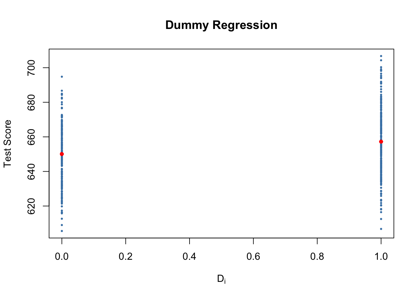
With \(D\) as the regressor, it is not useful to think of \(\beta_1\) as a slope parameter since \(D_i \in \{0,1\}\), i.e., we only observe two discrete values instead of a continuum of regressor values. There is no continuous line depicting the conditional expectation function \(E(TestScore_i | D_i)\) since this function is solely defined for \(x\)-positions \(0\) and \(1\).
Therefore, the interpretation of the coefficients in this regression model is as follows:
\(E(Y_i | D_i = 0) = \beta_0\), so \(\beta_0\) is the expected test score in districts where \(D_i=0\) and \(STR\) is above \(20\).
\(E(Y_i | D_i = 1) = \beta_0 + \beta_1\) or, using the result above, \(\beta_1 = E(Y_i | D_i = 1) - E(Y_i | D_i = 0)\). Thus, \(\beta_1\) is the difference in group-specific expectations, i.e., the difference in expected test score between districts with \(STR < 20\) and those with \(STR \geq 20\).
We will now use R to estimate the dummy regression model as defined by the equations (5.2) and (5.3) .
# estimate the dummy regression model
dummy_model <- lm(score ~ D, data = CASchools)
summary(dummy_model)
#>
#> Call:
#> lm(formula = score ~ D, data = CASchools)
#>
#> Residuals:
#>     Min      1Q  Median      3Q     Max
#> -50.496 -14.029  -0.346  12.884  49.504
#>
#> Coefficients:
#>             Estimate Std. Error t value Pr(>|t|)
#> (Intercept)  650.077      1.393 466.666  < 2e-16 ***
#> DTRUE          7.169      1.847   3.882  0.00012 ***
#> ---
#> Signif. codes:  0 '***' 0.001 '**' 0.01 '*' 0.05 '.' 0.1 ' ' 1
#>
#> Residual standard error: 18.74 on 418 degrees of freedom
#> Multiple R-squared:  0.0348, Adjusted R-squared:  0.0325
#> F-statistic: 15.07 on 1 and 418 DF, p-value: 0.0001202The vector CASchools$D has the type logical (to see this, use typeof(CASchools$D)) which is shown in the output of summary(dummy_model): the label DTRUE states that all entries TRUE are coded as 1 and all entries FALSE are coded as 0. Thus, the interpretation of the coefficient DTRUE is same as stated above for \(\beta_1\).
One can see that the expected test score in districts with \(STR < 20\) (\(D_i = 1\)) is predicted to be \(650.1 + 7.17 = 657.27\) while districts with \(STR \geq 20\) (\(D_i = 0\)) are expected to have an average test score of only \(650.1\).
Group specific predictions can be added to the plot by execution of the following code chunk.
# add group specific predictions to the plot
points(x = CASchools$D,
       y = predict(dummy_model),
       col = "red",
       pch = 20)
Here we use the function predict() to obtain estimates of the group specific means. The red dots represent these sample group averages. Accordingly, \(\hat{\beta}_1 = 7.17\) can be seen as the difference in group averages.
summary(dummy_model) also answers the question whether there is a statistically significant difference in group means. This in turn would support the hypothesis that students perform differently when they are taught in small classes. We can assess this by a two-tailed test of the hypothesis \(H_0: \beta_1 = 0\). Conveniently, the \(t\)-statistic and the corresponding \(p\)-value for this test are computed by summary().
Since t value \(= 3.88 > 1.96\), we reject the null hypothesis at the \(5\%\) level of significance. The same conclusion results when using the \(p\)-value, which reports significance up to the \(0.00012\%\) level.
As done with linear_model, we may alternatively use the function confint() to compute a \(95\%\) confidence interval for the true difference in means and see if the hypothesized value is an element of this confidence set.
# confidence intervals for coefficients in the dummy regression model
confint(dummy_model)
#>                  2.5 %    97.5 %
#> (Intercept) 647.338594 652.81500
#> DTRUE         3.539562  10.79931
We reject the hypothesis that there is no difference between group means at the \(5\%\) significance level since \(\beta_{1,0} = 0\) lies outside of \([3.54, 10.8]\), the \(95\%\) confidence interval for the coefficient on \(D\).