8.2 Nonlinear Functions of a Single Independent Variable
Polynomials
The approach used to obtain a quadratic model can be generalized to polynomial models of arbitrary degree \(r\), \[Y_i = \beta_0 + \beta_1 X_i + \beta_2 X_i^2 + \cdots + \beta_r X_i^r + u_i.\]
A cubic model for instance can be estimated in the same way as the quadratic model; we just have to use a polynomial of degree \(r=3\) in income. This is conveniently done using the function poly().
# estimate a cubic model
cubic_model <- lm(score ~ poly(income, degree = 3, raw = TRUE), data = CASchools)
poly() generates orthogonal polynomials which are orthogonal to the constant by default. Here, we set raw = TRUE such that raw polynomials are evaluated, see ?poly.
In practice the question will arise which polynomial order should be chosen. First, similarly as for \(r=2\), we can test the null hypothesis that the true relation is linear against the alternative hypothesis that the relationship is a polynomial of degree \(r\):
\[ H_0: \beta_2=0, \ \beta_3=0,\dots,\beta_r=0 \ \ \ \text{vs.} \ \ \ H_1: \text{at least one} \ \beta_j\neq0, \ j=2,\dots,r. \]
This is a joint null hypothesis with \(r-1\) restrictions so it can be tested using the \(F\)-test presented in Chapter 7. linearHypothesis() can be used to conduct such tests. For example, we may test the null of a linear model against the alternative of a polynomial of a maximal degree \(r=3\) as follows.
# test the hypothesis of a linear model against quadratic or polynomial
# alternatives

# set up hypothesis matrix
R <- rbind(c(0, 0, 1, 0),
            c(0, 0, 0, 1))

# do the test
linearHypothesis(cubic_model,
                 hypothesis.matrix = R,
                 white.adj = "hc1")
#>
#> Linear hypothesis test:
#> poly(income, degree = 3, raw = TRUE)2 = 0
#> poly(income, degree = 3, raw = TRUE)3 = 0
#>
#> Model 1: restricted model
#> Model 2: score ~ poly(income, degree = 3, raw = TRUE)
#>
#> Note: Coefficient covariance matrix supplied.
#>
#>   Res.Df Df      F    Pr(>F)
#> 1    418
#> 2    416  2 37.691 9.043e-16 ***
#> ---
#> Signif. codes:  0 '***' 0.001 '**' 0.01 '*' 0.05 '.' 0.1 ' ' 1
We provide a hypothesis matrix as the argument hypothesis.matrix. This is useful when the coefficients have long names, as is the case here due to using poly(), or when the restrictions include multiple coefficients. How the hypothesis matrix \(\mathbf{R}\) is interpreted by linearHypothesis() is best seen using matrix algebra:
For the two linear constraints above, we have
\[\begin{align*}
\mathbf{R}\boldsymbol{\beta} =& \mathbf{s} \\
\\
\begin{pmatrix}
0 & 0 & 1 & 0 \\
0 & 0 & 0 & 1
\end{pmatrix}
\begin{pmatrix}
\beta_0 \\
\beta_1 \\
\beta_2 \\
\beta_3 \\
\end{pmatrix} =&
\begin{pmatrix}
0 \\
0
\end{pmatrix} =>
\begin{pmatrix}
\beta_2 \\
\beta_3
\end{pmatrix} =
\begin{pmatrix}
0 \\
0
\end{pmatrix}.
\end{align*}\]
linearHypothesis() uses the zero vector for \(\mathbf{s}\) by default, see ?linearHypothesis.
The \(p\)-value for the test is very small so that we reject the null hypothesis. However, this does not tell us which \(r\) to choose. In practice, one approach to determine the degree of the polynomial is to use sequential testing:
- Estimate a polynomial model for some maximum value \(r\).
- Use a \(t\)-test to test \(\beta_r = 0\). Rejection of the null means that \(X^r\) belongs in the regression equation.
- Acceptance of the null in step 2 means that \(X^r\) can be eliminated from the model. Continue by repeating step 1 with order \(r-1\) and test whether \(\beta_{r-1}=0\). If the test rejects, use a polynomial model of order \(r-1\).
- If the test from step 3 rejects, continue with the procedure until the coefficient on the highest power is statistically significant.
There is no unambiguous guideline on how to choose \(r\) in step one. However, as pointed out in Stock and Watson (2015), economic data is often smooth such that it is appropriate to choose small orders like \(2\), \(3\), or \(4\).
We will demonstrate how to apply sequential testing by the example of the cubic model.
summary(cubic_model)
#>
#> Call:
#> lm(formula = score ~ poly(income, degree = 3, raw = TRUE), data = CASchools)
#>
#> Residuals:
#>    Min     1Q Median     3Q    Max
#> -44.28  -9.21   0.20   8.32  31.16
#>
#> Coefficients:
#>                                         Estimate Std. Error t value Pr(>|t|)
#> (Intercept)                            6.001e+02  5.830e+00 102.937  < 2e-16
#> poly(income, degree = 3, raw = TRUE)1  5.019e+00  8.595e-01   5.839 1.06e-08
#> poly(income, degree = 3, raw = TRUE)2 -9.581e-02  3.736e-02  -2.564   0.0107
#> poly(income, degree = 3, raw = TRUE)3  6.855e-04  4.720e-04   1.452   0.1471
#>
#> (Intercept)                           ***
#> poly(income, degree = 3, raw = TRUE)1 ***
#> poly(income, degree = 3, raw = TRUE)2 *
#> poly(income, degree = 3, raw = TRUE)3
#> ---
#> Signif. codes:  0 '***' 0.001 '**' 0.01 '*' 0.05 '.' 0.1 ' ' 1
#>
#> Residual standard error: 12.71 on 416 degrees of freedom
#> Multiple R-squared:  0.5584, Adjusted R-squared:  0.5552
#> F-statistic: 175.4 on 3 and 416 DF,  p-value: < 2.2e-16
The estimated cubic model stored in cubic_model is
\[ \widehat{TestScore}_i = \underset{(5.83)}{600.1} + \underset{(0.86)}{5.02} \times income -\underset{(0.037)}{0.096} \times income^2 - \underset{(0.00047)}{0.00069} \times income^3. \]
The \(t\)-statistic on \(income^3\) is \(1.45\) so the null that the relationship is quadratic cannot be rejected, even at the \(10\%\) level. This is contrary to the result presented in the book which reports robust standard errors throughout, so we will also use robust variance-covariance estimation to reproduce these results.
# test the hypothesis using robust standard errors
coeftest(cubic_model, vcov. = vcovHC, type = "HC1")
#>
#> t test of coefficients:
#>
#>                                          Estimate  Std. Error  t value
#> (Intercept)                            6.0008e+02  5.1021e+00 117.6150
#> poly(income, degree = 3, raw = TRUE)1  5.0187e+00  7.0735e-01   7.0950
#> poly(income, degree = 3, raw = TRUE)2 -9.5805e-02  2.8954e-02  -3.3089
#> poly(income, degree = 3, raw = TRUE)3  6.8549e-04  3.4706e-04   1.9751
#>                                        Pr(>|t|)
#> (Intercept)                           < 2.2e-16 ***
#> poly(income, degree = 3, raw = TRUE)1 5.606e-12 ***
#> poly(income, degree = 3, raw = TRUE)2  0.001018 **
#> poly(income, degree = 3, raw = TRUE)3  0.048918 *
#> ---
#> Signif. codes:  0 '***' 0.001 '**' 0.01 '*' 0.05 '.' 0.1 ' ' 1
The reported standard errors have changed. Furthermore, the coefficient for income^3 is now significant at the \(5\%\) level. This means we reject the hypothesis that the regression function is quadratic against the alternative that it is cubic. Furthermore, we can also test if the coefficients for income^2 and income^3 are jointly significant using a robust version of the \(F\)-test.
# perform robust F-test
linearHypothesis(cubic_model,
                 hypothesis.matrix = R,
                 vcov. = vcovHC, type = "HC1")
#>
#> Linear hypothesis test:
#> poly(income, degree = 3, raw = TRUE)2 = 0
#> poly(income, degree = 3, raw = TRUE)3 = 0
#>
#> Model 1: restricted model
#> Model 2: score ~ poly(income, degree = 3, raw = TRUE)
#>
#> Note: Coefficient covariance matrix supplied.
#>
#>   Res.Df Df      F    Pr(>F)
#> 1    418
#> 2    416  2 29.678 8.945e-13 ***
#> ---
#> Signif. codes:  0 '***' 0.001 '**' 0.01 '*' 0.05 '.' 0.1 ' ' 1
With a \(p\)-value of \(8.945e-13\), i.e., much less than \(0.05\), the null hypothesis of linearity is rejected in favor of the alternative that the relationship is quadratic or cubic.
Interpretation of Coefficients in Nonlinear Regression Models
The coefficients in the polynomial regressions do not have a simple interpretation. Why? Think of a quadratic model: it is not helpful to think of the coefficient on \(X\) as the expected change in \(Y\) associated with a change in \(X\) holding the other regressors constant because \(X^2\) changes as \(X\) varies. This is also the case for other deviations from linearity, for example in models where regressors and/or the dependent variable are log-transformed. A way to approach this is to calculate the estimated effect on \(Y\) associated with a change in \(X\) for one or more values of \(X\). This idea is summarized in Key Concept 8.1.
Key Concept 8.1
The Expected Effect on \(Y\) for a Change in \(X_1\) in a Nonlinear Regression Model
Consider the nonlinear population regression model
\[ Y_i = f(X_{1i}, X_{2i}, \dots, X_{ki}) + u_i \ , \ i=1,\dots,n,\]
where \(f(X_{1i}, X_{2i}, \dots, X_{ki})\) is the population regression function and \(u_i\) is the error term.
Denote by \(\Delta Y\) the expected change in \(Y\) associated with \(\Delta X_1\), the change in \(X_1\) while holding \(X_2, \cdots , X_k\) constant. That is, the expected change in \(Y\) is the difference
\[\Delta Y = f(X_1 + \Delta X_1, X_2, \cdots, X_k) - f(X_1, X_2, \cdots, X_k).\]
The estimator of this unknown population difference is the difference between the predicted values for these two cases. Let \(\hat{f}(X_1, X_2, \cdots, X_k)\) be the predicted value of of \(Y\) based on the estimator \(\hat{f}\) of the population regression function. Then the predicted change in \(Y\) is
\[\Delta \widehat{Y} = \hat{f}(X_1 + \Delta X_1, X_2, \cdots, X_k) - \hat{f}(X_1, X_2, \cdots, X_k).\]For example, we may ask the following: what is the predicted change in test scores associated with a one unit change (i.e., \(\$1000\)) in income, based on the estimated quadratic regression function
\[\widehat{TestScore} = 607.3 + 3.85 \times income - 0.0423 \times income^2\ ?\]
Because the regression function is quadratic, this effect depends on the initial district income. We therefore consider two cases:
An increase in district income form \(10\) to \(11\) (from \(\$10000\) per capita to \(\$11000\)).
An increase in district income from \(40\) to \(41\) (that is from \(\$40000\) to \(\$41000\)).
In order to obtain the \(\Delta \widehat{Y}\) associated with a change in income form \(10\) to \(11\), we use the following formula:
\[\Delta \widehat{Y} = \left(\hat{\beta}_0 + \hat{\beta}_1 \times 11 + \hat{\beta}_2 \times 11^2\right) - \left(\hat{\beta}_0 + \hat{\beta}_1 \times 10 + \hat{\beta}_2 \times 10^2\right). \] To compute \(\widehat{Y}\) using R we may use predict().
# compute and assign the quadratic model
quadratic_model <- lm(score ~ income + I(income^2), data = CASchools)

# set up data for prediction
new_data <- data.frame(income = c(10, 11))

# do the prediction
Y_hat <- predict(quadratic_model, newdata = new_data)

# compute the difference
diff(Y_hat)
#>        2
#> 2.962517
Analogously we can compute the effect of a change in district income from \(40\) to \(41\):
# set up data for prediction
new_data <- data.frame(income = c(40, 41))

# do the prediction
Y_hat <- predict(quadratic_model, newdata = new_data)

# compute the difference
diff(Y_hat)
#>         2
#> 0.4240097
So for the quadratic model, the expected change in \(TestScore\) induced by an increase in \(income\) from \(10\) to \(11\) is about \(2.96\) points but an increase in \(income\) from \(40\) to \(41\) increases the predicted score by only \(0.42\). Hence, the slope of the estimated quadratic regression function is steeper at low levels of income than at higher levels.
Logarithms
Another way to specify a nonlinear regression function is to use the natural logarithm of \(Y\) and/or \(X\). Logarithms convert changes in variables into percentage changes. This is convenient as many relationships are naturally expressed in terms of percentages.
There are three different cases in which logarithms might be used.
Transform \(X\) to its logarithm, but not \(Y\).
Analogously we can transform \(Y\) to its logarithm but leave \(X\) at level.
Both \(Y\) and \(X\) are transformed to their logarithms.
The interpretation of the regression coefficients is different in each case.
Case I: \(X\) is in Logarithm, \(Y\) is not.
The regression model then is \[Y_i = \beta_0 + \beta_1 \times \ln(X_i) + u_i \text{, } i=1,...,n. \] Similar as for polynomial regressions, we do not have to create a new variable before using lm(). We can simply adjust the formula argument of lm() to tell R that the log-transformation of a variable should be used.
# estimate a level-log model
LinearLog_model <- lm(score ~ log(income), data = CASchools)

# compute robust summary
coeftest(LinearLog_model,
         vcov = vcovHC, type = "HC1")
#>
#> t test of coefficients:
#>
#>             Estimate Std. Error t value  Pr(>|t|)
#> (Intercept) 557.8323     3.8399 145.271 < 2.2e-16 ***
#> log(income)  36.4197     1.3969  26.071 < 2.2e-16 ***
#> ---
#> Signif. codes:  0 '***' 0.001 '**' 0.01 '*' 0.05 '.' 0.1 ' ' 1
Hence, the estimated regression function is
\[\widehat{TestScore} = 557.8 + 36.42 \times \ln(income).\]
Let us draw a plot of this function.
# draw a scatterplot
plot(score ~ income,
     col = "steelblue",
     pch = 20,
     data = CASchools,
     ylab="Score",
     xlab="Income",
     main = "Linear-Log Regression Line")

# add the linear-log regression line
order_id  <- order(CASchools$income)

lines(CASchools$income[order_id],
      fitted(LinearLog_model)[order_id],
      col = "red",
      lwd = 2)
legend("bottomright",legend = "Linear-log line",lwd = 2,col ="red")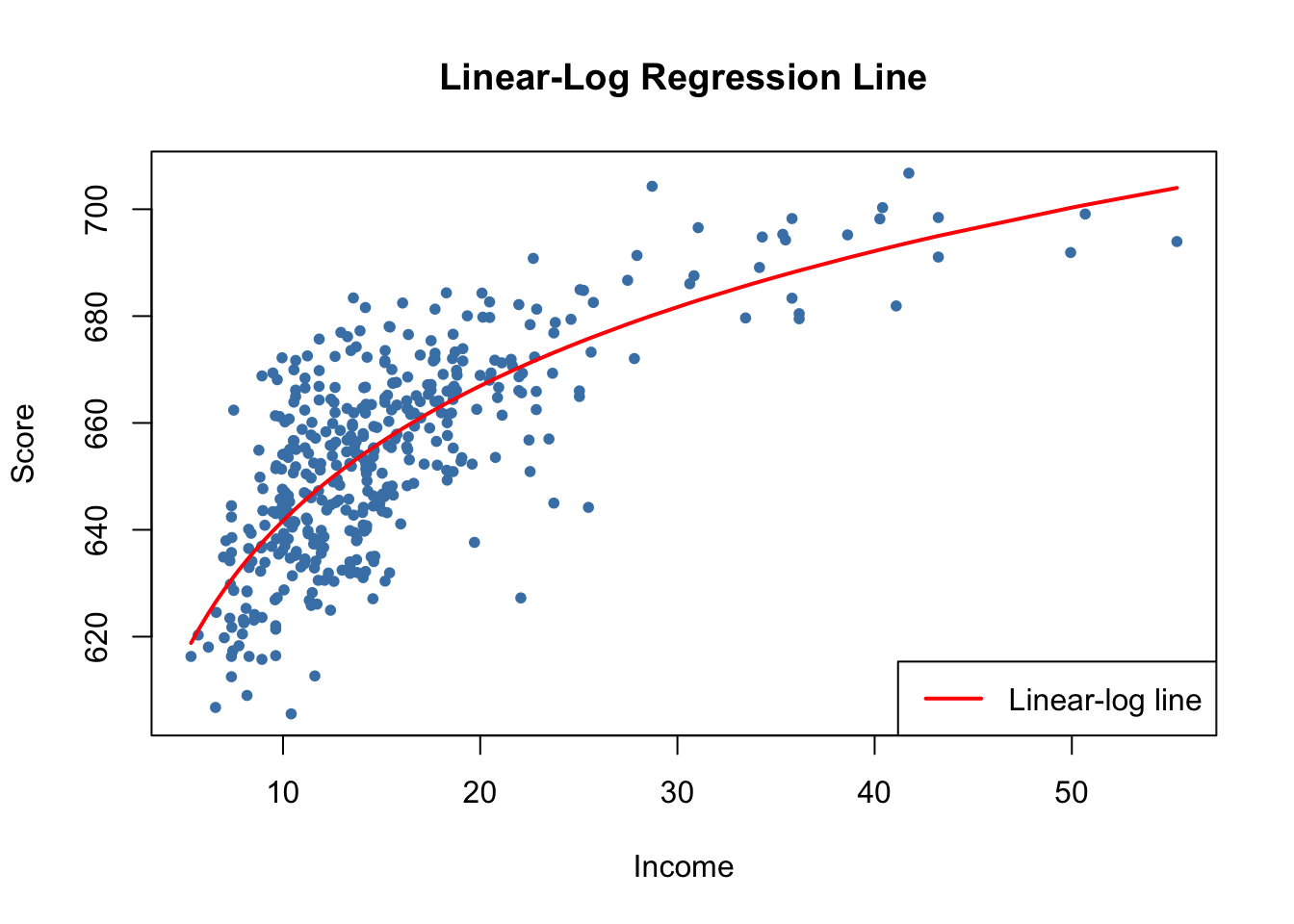
We can interpret \(\hat{\beta}_1\) as follows: a \(1\%\) increase in income is associated with an increase in test scores of \(0.01 \times 36.42 = 0.36\) points. In order to get the estimated effect of a one unit change in income (that is, a change in the original units, thousands of dollars) on test scores, the method presented in Key Concept 8.1 can be used.
# set up new data
new_data <- data.frame(income = c(10, 11, 40, 41))

# predict the outcomes
Y_hat <- predict(LinearLog_model, newdata = new_data)

# compute the expected difference
Y_hat_matrix <- matrix(Y_hat, nrow = 2, byrow = TRUE)
Y_hat_matrix[, 2] - Y_hat_matrix[, 1]
#> [1] 3.471166 0.899297
By setting nrow = 2 and byrow = TRUE in matrix(), we ensure that Y_hat_matrix is a \(2\times2\) matrix filled row-wise with the entries of Y_hat.
The estimated model states that for an income increase from \(\$10000\) to \(\$11000\), test scores increase by an expected amount of \(3.47\) points. When income increases from \(\$40000\) to \(\$41000\), the expected increase in test scores is only about \(0.90\) points.
Case II: \(Y\) is in Logarithm, \(X\) is not
There are cases where it is useful to regress \(\ln(Y)\).
The corresponding regression model then is
\[ \ln(Y_i) = \beta_0 + \beta_1 \times X_i + u_i , \ \ i=1,...,n. \]
# estimate a log-linear model
LogLinear_model <- lm(log(score) ~ income, data = CASchools)

# obtain a robust coefficient summary
coeftest(LogLinear_model,
         vcov = vcovHC, type = "HC1")
#>
#> t test of coefficients:
#>
#>               Estimate Std. Error  t value  Pr(>|t|)
#> (Intercept) 6.43936234 0.00289382 2225.210 < 2.2e-16 ***
#> income      0.00284407 0.00017509   16.244 < 2.2e-16 ***
#> ---
#> Signif. codes:  0 '***' 0.001 '**' 0.01 '*' 0.05 '.' 0.1 ' ' 1
The estimated regression function is \[\widehat{\ln(TestScore)} = 6.439 + 0.00284 \times income.\] An increase in district income by \(\$1000\) is expected to increase test scores by \(100\times 0.00284 \% = 0.284\%\).
When the dependent variable in logarithm, one cannot simply use \(e^{\log(\cdot)}\) to transform predictions back to the original scale, see page of the book.
Case III: \(X\) and \(Y\) are in Logarithms
The log-log regression model is \[\ln(Y_i) = \beta_0 + \beta_1 \times \ln(X_i) + u_i, \ \ i=1,...,n.\]
# estimate the log-log model
LogLog_model <- lm(log(score) ~ log(income), data = CASchools)

# print robust coefficient summary to the console
coeftest(LogLog_model,
         vcov = vcovHC, type = "HC1")
#>
#> t test of coefficients:
#>
#>              Estimate Std. Error  t value  Pr(>|t|)
#> (Intercept) 6.3363494  0.0059246 1069.501 < 2.2e-16 ***
#> log(income) 0.0554190  0.0021446   25.841 < 2.2e-16 ***
#> ---
#> Signif. codes:  0 '***' 0.001 '**' 0.01 '*' 0.05 '.' 0.1 ' ' 1
The estimated regression function hence is \[\widehat{\ln(TestScore)} = 6.336 + 0.0554 \times \ln(income).\] In a log-log model, a \(1\%\) change in \(X\) is associated with an estimated \(\hat\beta_1 \%\) change in \(Y\).
We now reproduce Figure 8.5 of the book.
# generate a scatterplot
plot(log(score) ~ income,
     col = "steelblue",
     pch = 20,
     data = CASchools,
     ylab="log(Score)",
     xlab="Income",
     main = "Log-Linear Regression Function")

# add the log-linear regression line
order_id  <- order(CASchools$income)

lines(CASchools$income[order_id],
      fitted(LogLinear_model)[order_id],
      col = "red",
      lwd = 2)

# add the log-log regression line
lines(sort(CASchools$income),
      fitted(LogLog_model)[order(CASchools$income)],
      col = "green",
      lwd = 2)

# add a legend
legend("bottomright",
       legend = c("log-linear model", "log-log model"),
       lwd = 2,
       col = c("red", "green"))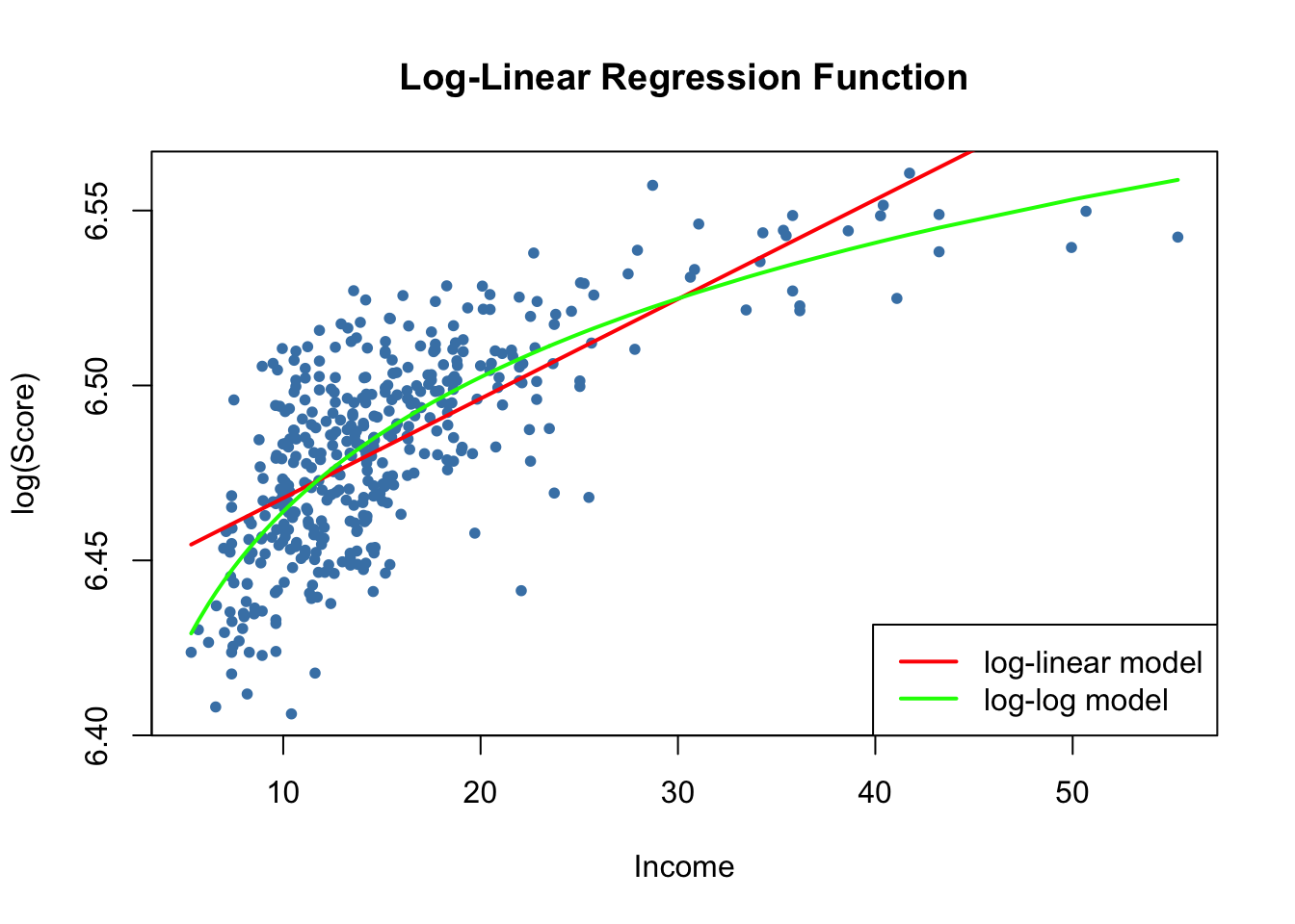
Key Concept 8.2 summarizes the three logarithmic regression models.
Key Concept 8.2
Logarithms in Regression: Three Cases
Logarithms can be used to transform the dependent variable \(Y\) or the independent variable \(X\), or both (the variable being transformed must be positive). The following table summarizes these three cases and the interpretation of the regression coefficient \(\beta_1\). In each case, \(\beta_1\), can be estimated by applying OLS after taking the logarithm(s) of the dependent and/or the independent variable.
| Case | Model Specification | Interpretation of \(\beta_1\) |
|---|---|---|
| \((I)\) | \(Y_i = \beta_0 + \beta_1 \ln(X_i) + u_i\) | A \(1 \%\) change in \(X\) is associated with a change in \(Y\) of \(0.01 \times \beta_1\). |
| \((II)\) | \(\ln(Y_i) = \beta_0 + \beta_1 X_i + u_i\) | A change in \(X\) by one unit (\(\Delta X = 1\)) is associated with a \(100 \times \beta_1 \%\) change in \(Y\). |
| \((III)\) | \(\ln(Y_i) = \beta_0 + \beta_1 \ln(X_i) + u_i\) | A \(1\%\) change in \(X\) is associated with a \(\beta_1\%\) change in \(Y\), so \(\beta_1\) is the elasticity of \(Y\) with respect to \(X\). |
Of course we can also estimate a polylog model like
\[ TestScore_i = \beta_0 + \beta_1 \times \ln(income_i) + \beta_2 \times \ln(income_i)^2 + \beta_3 \times \ln(income_i)^3 + u_i, \]
which models the dependent variable \(TestScore\) by a third-degree polynomial of the log-transformed regressor \(income\).
# estimate the polylog model
polyLog_model <- lm(score ~ log(income) + I(log(income)^2) + I(log(income)^3),
                    data = CASchools)

# print robust summary to the console
coeftest(polyLog_model,
         vcov = vcovHC, type = "HC1")
#>
#> t test of coefficients:
#>
#>                  Estimate Std. Error t value  Pr(>|t|)
#> (Intercept)      486.1341    79.3825  6.1239 2.115e-09 ***
#> log(income)      113.3820    87.8837  1.2901    0.1977
#> I(log(income)^2) -26.9111    31.7457 -0.8477    0.3971
#> I(log(income)^3)   3.0632     3.7369  0.8197    0.4128
#> ---
#> Signif. codes:  0 '***' 0.001 '**' 0.01 '*' 0.05 '.' 0.1 ' ' 1
Comparing by \(\bar{R}^2\) we find that, leaving out the log-linear model, all models have a similar adjusted fit. In the class of polynomial models, the cubic specification has the highest \(\bar{R}^2\) whereas the linear-log specification is the best of the log-models.
# compute the adj. R^2 for the nonlinear models
adj_R2 <-rbind("quadratic" = summary(quadratic_model)$adj.r.squared,
               "cubic" = summary(cubic_model)$adj.r.squared,
               "LinearLog" = summary(LinearLog_model)$adj.r.squared,
               "LogLinear" = summary(LogLinear_model)$adj.r.squared,
               "LogLog" = summary(LogLog_model)$adj.r.squared,
               "polyLog" = summary(polyLog_model)$adj.r.squared)

# assign column names
colnames(adj_R2) <- "adj_R2"

adj_R2
#>              adj_R2
#> quadratic 0.5540444
#> cubic     0.5552279
#> LinearLog 0.5614605
#> LogLinear 0.4970106
#> LogLog    0.5567251
#> polyLog   0.5599944
Let us now compare the cubic and the linear-log model by plotting the corresponding estimated regression functions.
# generate a scatterplot
plot(score ~ income,
     data = CASchools,
     col = "steelblue",
     pch = 20,
     ylab="Score",
     xlab="Income",
     main = "Linear-Log and Cubic Regression Functions")

# add the linear-log regression line
order_id  <- order(CASchools$income)

lines(CASchools$income[order_id],
      fitted(LinearLog_model)[order_id],
      col = "darkgreen",
      lwd = 2)

# add the cubic regression line
lines(x = CASchools$income[order_id],
      y = fitted(cubic_model)[order_id],
      col = "red",
      lwd = 2)
# add a legend
legend("bottomright",
       legend = c("Linear-Log model", "Cubic model"),
       lwd = 2,
       col = c("darkgreen", "red"))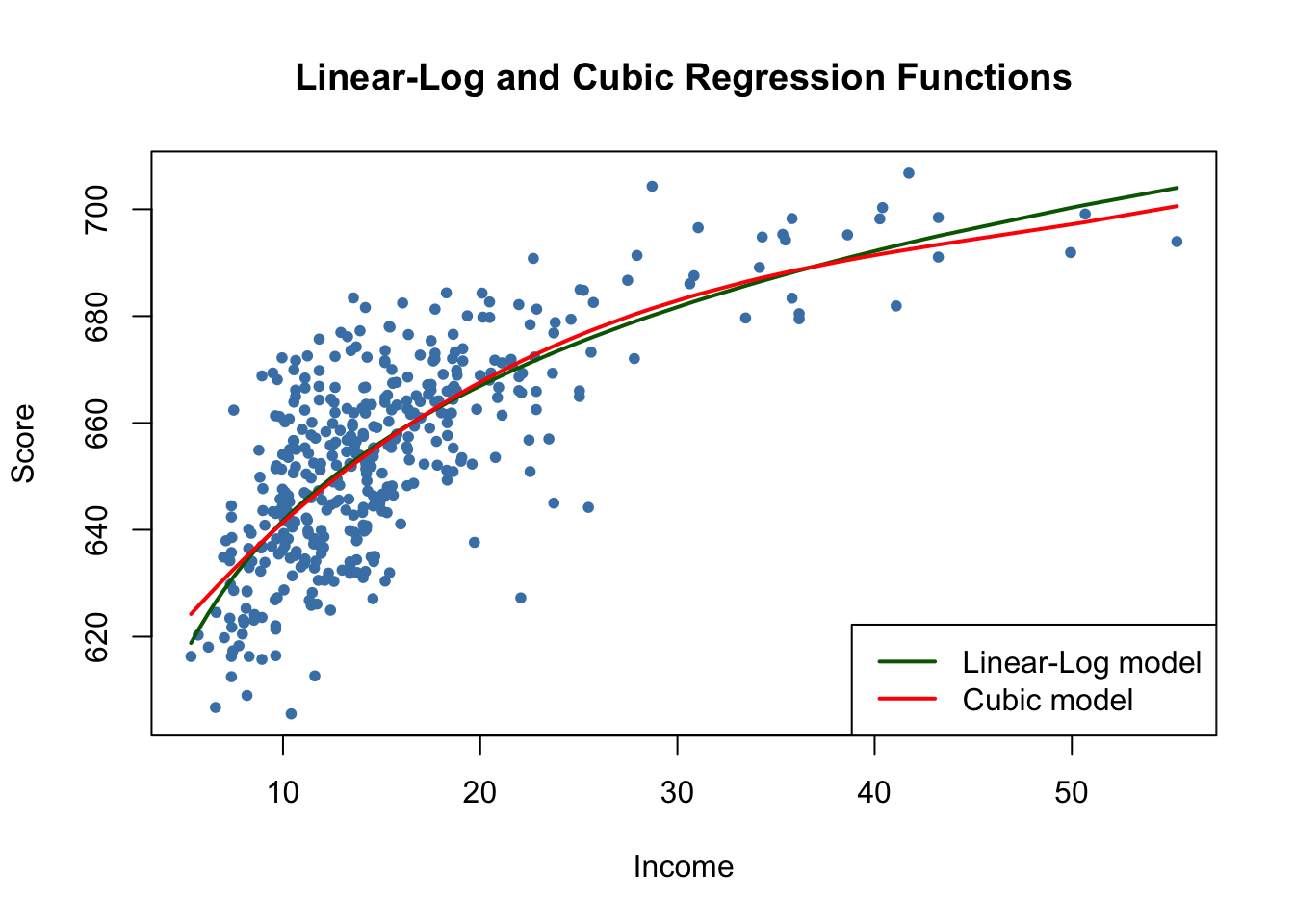
Both regression lines look nearly identical. Altogether the linear-log model may be preferable since it is more parsimonious in terms of regressors: it does not include higher-degree polynomials.