11.2 Probit and Logit Regression
The linear probability model has a major flaw: it assumes the conditional probability function to be linear. This does not restrict \(P(Y=1\vert X_1,\dots,X_k)\) to lie between \(0\) and \(1\). We can easily see this in our reproduction of Figure 11.1 of the book: for \(P/I \ ratio \geq 1.75\), (11.2) predicts the probability of a mortgage application denial to be bigger than \(1\). For applications with \(P/I \ ratio\) close to \(0\), the predicted probability of denial is even negative so that the model has no meaningful interpretation here.
This circumstance calls for an approach that uses a nonlinear function to model the conditional probability function of a binary dependent variable. Commonly used methods are Probit and Logit regression.
Probit Regression
In Probit regression, the cumulative standard normal distribution function \(\Phi(\cdot)\) is used to model the regression function when the dependent variable is binary, that is, we assume \[\begin{align} E(Y\vert X) = P(Y=1\vert X) = \Phi(\beta_0 + \beta_1 X). \tag{11.4} \end{align}\]
\(\beta_0 + \beta_1 X\) in (11.4) plays the role of a quantile \(z\). Remember that \[\Phi(z) = P(Z \leq z) \ , \ Z \sim \mathcal{N}(0,1),\] such that the Probit coefficient \(\beta_1\) in (11.4) is the change in \(z\) associated with a one unit change in \(X\). Although the effect on \(z\) of a change in \(X\) is linear, the link between \(z\) and the dependent variable \(Y\) is nonlinear since \(\Phi\) is a nonlinear function of \(X\).
Since the dependent variable is a nonlinear function of the regressors, the coefficient on \(X\) has no simple interpretation. According to Key Concept 8.1, the expected change in the probability that \(Y=1\) due to a change in \(P/I \ ratio\) can be computed as follows:
- Compute the predicted probability that \(Y=1\) for the original value of \(X\).
- Compute the predicted probability that \(Y=1\) for \(X + \Delta X\).
- Compute the difference between both the predicted probabilities.
Of course, we can generalize (11.4) to Probit regression with multiple regressors to mitigate the risk of facing omitted variable bias. Probit regression essentials are summarized in Key Concept 11.2.
Key Concept 11.2
Probit Model, Predicted Probabilities and Estimated Effects
Assume that \(Y\) is a binary variable. The model
\[ Y= \beta_0 + \beta_1 + X_1 + \beta_2 X_2 + \dots + \beta_k X_k + u \] with \[P(Y = 1 \vert X_1, X_2, \dots ,X_k) = \Phi(\beta_0 + \beta_1 + X_1 + \beta_2 X_2 + \dots + \beta_k X_k)\] is the population Probit model with multiple regressors \(X_1, X_2, \dots, X_k\) and \(\Phi(\cdot)\) is the cumulative standard normal distribution function.
The predicted probability that \(Y=1\) given \(X_1, X_2, \dots, X_k\) can be calculated in two steps:
Compute \(z = \beta_0 + \beta_1 X_1 + \beta_2 X_2 + \dots + \beta_k X_k\),
Look up \(\Phi(z)\) by calling pnorm().
\(\beta_j\) is the effect on \(z\) of a one unit change in regressor \(X_j\), holding constant all other \(k-1\) regressors.
The effect on the predicted probability of a change in a regressor can be computed as in Key Concept 8.1.
In R, Probit models can be estimated using the function glm() from the package stats. Using the argument family we specify that we want to use a Probit link function.
We now estimate a simple Probit model of the probability of a mortgage denial.
# estimate the simple probit model
denyprobit <- glm(deny ~ pirat,
                  family = binomial(link = "probit"),
                  data = HMDA)

coeftest(denyprobit, vcov. = vcovHC, type = "HC1")
#>
#> z test of coefficients:
#>
#>             Estimate Std. Error  z value  Pr(>|z|)
#> (Intercept) -2.19415    0.18901 -11.6087 < 2.2e-16 ***
#> pirat        2.96787    0.53698   5.5269 3.259e-08 ***
#> ---
#> Signif. codes:  0 '***' 0.001 '**' 0.01 '*' 0.05 '.' 0.1 ' ' 1
The estimated model is
\[\begin{align} \widehat{P(deny\vert P/I \ ratio}) = \Phi(-\underset{(0.19)}{2.19} + \underset{(0.54)}{2.97} P/I \ ratio). \tag{11.5} \end{align}\]
Just as in the linear probability model we find that the relation between the probability of denial and the payments-to-income ratio is positive and that the corresponding coefficient is highly significant.
The following code chunk reproduces Figure 11.2 of the book.
# plot data
plot(x = HMDA$pirat,
     y = HMDA$deny,
     main = "Probit Model of the Probability of Denial, Given P/I Ratio",
     xlab = "P/I ratio",
     ylab = "Deny",
     pch = 20,
     ylim = c(-0.4, 1.4),
     cex.main = 0.85)

# add horizontal dashed lines and text
abline(h = 1, lty = 2, col = "darkred")
abline(h = 0, lty = 2, col = "darkred")
text(2.5, 0.9, cex = 0.8, "Mortgage denied")
text(2.5, -0.1, cex= 0.8, "Mortgage approved")

# add estimated regression line
x <- seq(0, 3, 0.01)
y <- predict(denyprobit, list(pirat = x), type = "response")

lines(x, y, lwd = 1.5, col = "steelblue")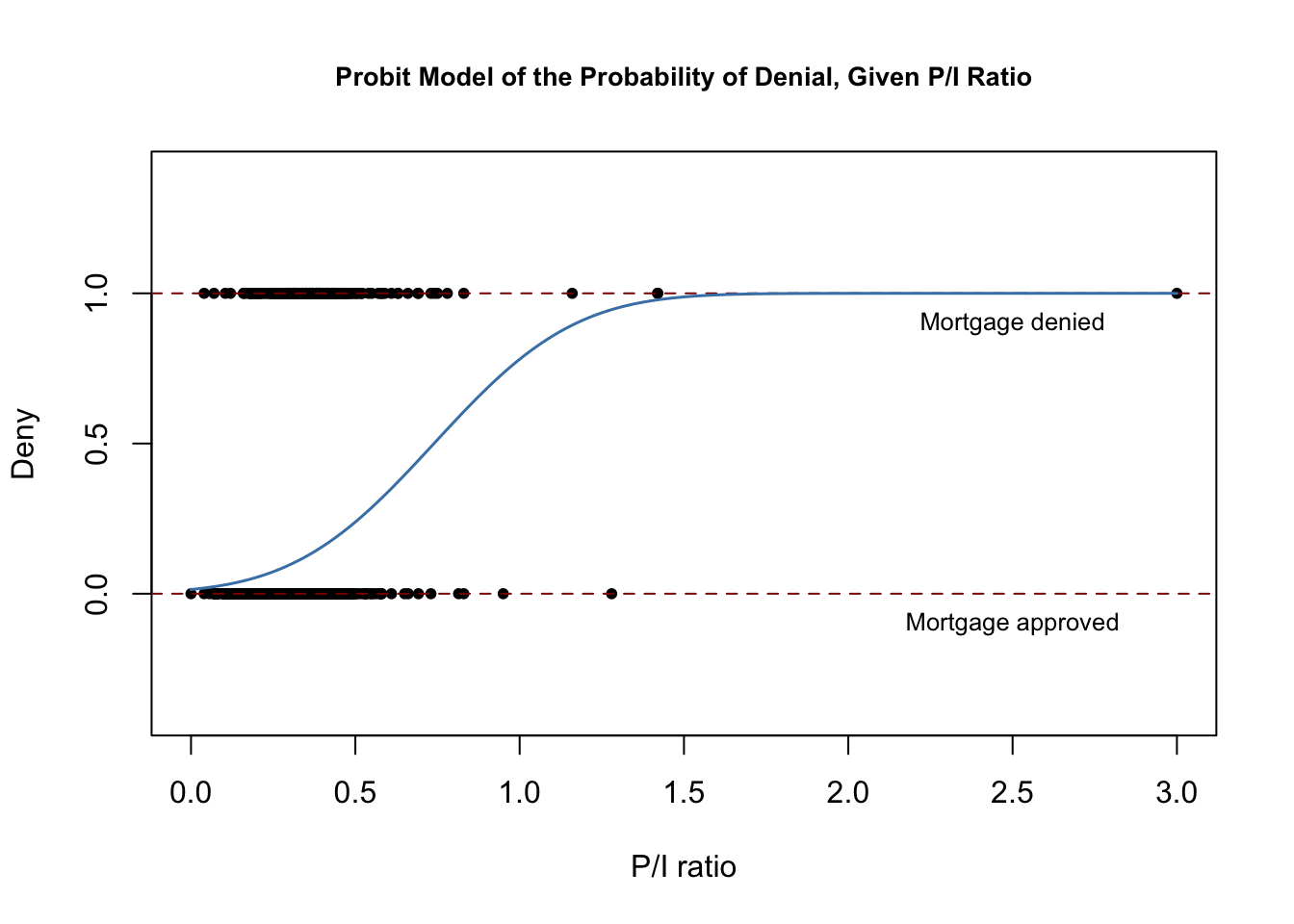
The estimated regression function has a stretched “S”-shape which is typical for the CDF of a continuous random variable with symmetric PDF like that of a normal random variable. The function is clearly nonlinear and flattens out for large and small values of \(P/I \ ratio\). The functional form thus also ensures that the predicted conditional probabilities of a denial lie between \(0\) and \(1\).
We use predict() to compute the predicted change in the denial probability when \(P/I \ ratio\) is increased from \(0.3\) to \(0.4\).
# 1. compute predictions for P/I ratio = 0.3, 0.4
predictions <- predict(denyprobit,
                       newdata = data.frame("pirat" = c(0.3, 0.4)),
                       type = "response")

# 2. Compute difference in probabilities
diff(predictions)
#>          2
#> 0.06081433
We find that an increase in the payment-to-income ratio from \(0.3\) to \(0.4\) is predicted to increase the probability of denial by approximately \(6.1\%\).
We continue by using an augmented Probit model to estimate the effect of race on the probability of a mortgage application denial.
#As a remainder, we have renamed the variable "afam" to "black" in Chapter 11.1
#colnames(HMDA)[colnames(HMDA) == "afam"] <- "black"
#We continue by using an augmented
denyprobit2 <- glm(deny ~ pirat + black,
                   family = binomial(link = "probit"),
                   data = HMDA)

coeftest(denyprobit2, vcov. = vcovHC, type = "HC1")
#>
#> z test of coefficients:
#>
#>              Estimate Std. Error  z value  Pr(>|z|)
#> (Intercept) -2.258787   0.176608 -12.7898 < 2.2e-16 ***
#> pirat        2.741779   0.497673   5.5092 3.605e-08 ***
#> blackyes     0.708155   0.083091   8.5227 < 2.2e-16 ***
#> ---
#> Signif. codes:  0 '***' 0.001 '**' 0.01 '*' 0.05 '.' 0.1 ' ' 1
The estimated model equation is
\[\begin{align} \widehat{P(deny\vert P/I \ ratio, black)} = \Phi (-\underset{(0.18)}{2.26} + \underset{(0.50)}{2.74} P/I \ ratio + \underset{(0.08)}{0.71} black). \tag{11.6} \end{align}\]
While all coefficients are highly significant, both the estimated coefficients on the payments-to-income ratio and the indicator for African American descent are positive. Again, the coefficients are difficult to interpret but they indicate that, first, African Americans have a higher probability of denial than white applicants, holding the payments-to-income ratio constant and second, applicants with a high payments-to-income ratio face a higher risk of being rejected.
How big is the estimated difference in denial probabilities between two hypothetical applicants with the same payments-to-income ratio? As before, we may use predict() to compute this difference.
# 1. Compute predictions for P/I ratio = 0.3
predictions <- predict(denyprobit2,
                       newdata = data.frame("black" = c("no", "yes"),
                                            "pirat" = c(0.3, 0.3)),
                       type = "response")

# 2. Compute difference in probabilities
diff(predictions)
#>         2
#> 0.1578117
In this case, the estimated difference in denial probabilities is about \(15.8\%\).
Logit Regression
Key Concept 11.3 summarizes the Logit regression function.
Key Concept 11.3
Logit Regression
The population Logit regression function is
\[\begin{align*} P(Y=1\vert X_1, X_2, \dots, X_k) =& \, F(\beta_0 + \beta_1 X_1 + \beta_2 X_2 + \dots + \beta_k X_k) \\ =& \, \frac{1}{1+e^{-(\beta_0 + \beta_1 X_1 + \beta_2 X_2 + \dots + \beta_k X_k)}}. \end{align*}\]
The idea is similar to Probit regression except that a different CDF is used: \[F(x) = \frac{1}{1+e^{-x}}\] is the CDF of a standard logistic distribution.
As for Probit regression, there is no simple interpretation of the model coefficients and it is best to consider predicted probabilities or differences in predicted probabilities. Here again, \(t\)-statistics and confidence intervals based on large sample normal approximations can be computed as usual.
It is fairly easy to estimate a Logit regression model using R.
denylogit <- glm(deny ~ pirat,
                 family = binomial(link = "logit"),
                 data = HMDA)

coeftest(denylogit, vcov. = vcovHC, type = "HC1")
#>
#> z test of coefficients:
#>
#>             Estimate Std. Error  z value  Pr(>|z|)
#> (Intercept) -4.02843    0.35898 -11.2218 < 2.2e-16 ***
#> pirat        5.88450    1.00015   5.8836 4.014e-09 ***
#> ---
#> Signif. codes:  0 '***' 0.001 '**' 0.01 '*' 0.05 '.' 0.1 ' ' 1
The subsequent code chunk reproduces Figure 11.3 of the book.
# plot data
plot(x = HMDA$pirat,
     y = HMDA$deny,
     main = "Probit and Logit Models of the Probability of Denial, Given P/I Ratio",
     xlab = "P/I ratio",
     ylab = "Deny",
     pch = 20,
     ylim = c(-0.4, 1.4),
     cex.main = 0.9)

# add horizontal dashed lines and text
abline(h = 1, lty = 2, col = "darkred")
abline(h = 0, lty = 2, col = "darkred")
text(2.5, 0.9, cex = 0.8, "Mortgage denied")
text(2.5, -0.1, cex= 0.8, "Mortgage approved")

# add estimated regression line of Probit and Logit models
x <- seq(0, 3, 0.01)
y_probit <- predict(denyprobit, list(pirat = x), type = "response")
y_logit <- predict(denylogit, list(pirat = x), type = "response")

lines(x, y_probit, lwd = 1.5, col = "steelblue")
lines(x, y_logit, lwd = 1.5, col = "black", lty = 2)

# add a legend
legend("topleft",
       horiz = TRUE,
       legend = c("Probit", "Logit"),
       col = c("steelblue", "black"),
       lty = c(1, 2))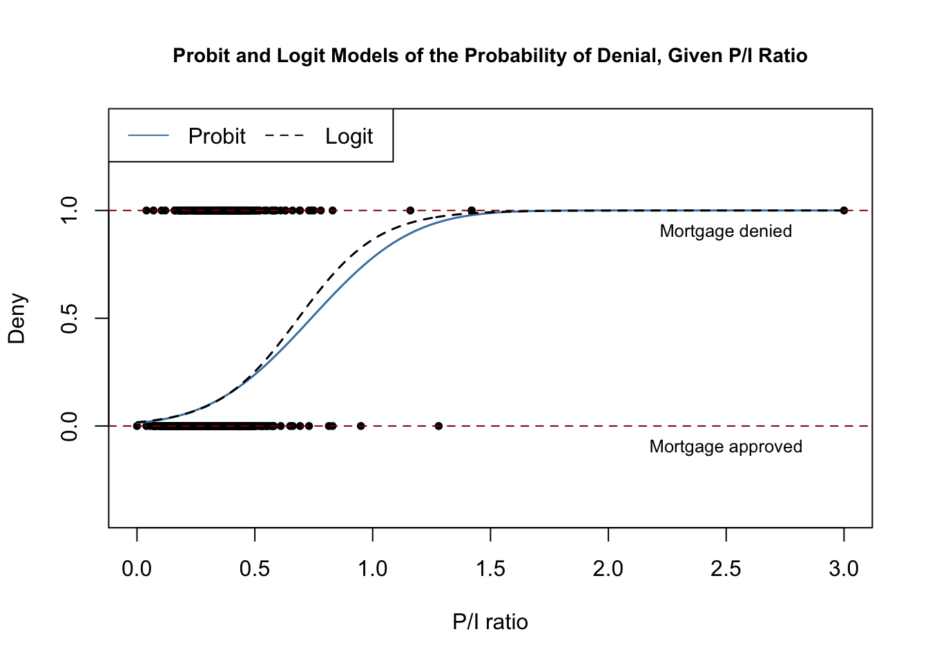
Both models produce very similar estimates of the probability that a mortgage application will be denied depending on the applicants payment-to-income ratio.
Following the book we extend the simple Logit model of mortgage denial with the additional regressor \(black\).
# estimate a Logit regression with multiple regressors
denylogit2 <- glm(deny ~ pirat + black,
                  family = binomial(link = "logit"),
                  data = HMDA)

coeftest(denylogit2, vcov. = vcovHC, type = "HC1")
#>
#> z test of coefficients:
#>
#>             Estimate Std. Error  z value  Pr(>|z|)
#> (Intercept) -4.12556    0.34597 -11.9245 < 2.2e-16 ***
#> pirat        5.37036    0.96376   5.5723 2.514e-08 ***
#> blackyes     1.27278    0.14616   8.7081 < 2.2e-16 ***
#> ---
#> Signif. codes:  0 '***' 0.001 '**' 0.01 '*' 0.05 '.' 0.1 ' ' 1
We obtain
\[\begin{align} \widehat{P(deny=1 \vert P/I ratio, black)} = F(-\underset{(0.35)}{4.13} + \underset{(0.96)}{5.37} P/I \ ratio + \underset{(0.15)}{1.27} black). \tag{11.7} \end{align}\]
As for the Probit model (11.6) all model coefficients are highly significant and we obtain positive estimates for the coefficients on \(P/I \ ratio\) and \(black\). For comparison we compute the predicted probability of denial for two hypothetical applicants that differ in race and have a \(P/I \ ratio\) of \(0.3\).
# 1. compute predictions for P/I ratio = 0.3
predictions <- predict(denylogit2,
                       newdata = data.frame("black" = c("no", "yes"),
                                            "pirat" = c(0.3, 0.3)),
                       type = "response")

predictions
#>          1          2
#> 0.07485143 0.22414592

# 2. Compute difference in probabilities
diff(predictions)
#>         2
#> 0.1492945
We find that the white applicant faces a denial probability of only \(7.5\%\), while the African American is rejected with a probability of \(22.4\%\), a difference of \(14.9\%\) points.
Comparison of the Models
The Probit model and the Logit model deliver only approximations to the unknown population regression function \(E(Y\vert X)\). It is not obvious how to decide which model to use in practice. The linear probability model has the clear drawback of not being able to capture the nonlinear nature of the population regression function and it may predict probabilities to lie outside the interval \([0,1]\). Probit and Logit models are harder to interpret but capture the nonlinearities better than the linear approach: both models produce predictions of probabilities that lie inside the interval \([0,1]\). Predictions of all three models are often close to each other. The book suggests to use the method that is easiest to use in the statistical software of choice. As we have seen, it is equally easy to estimate Probit and Logit model using R. We can therefore give no general recommendation which method to use.