3.7 Scatterplots, Sample Covariance and Sample Correlation
A scatter plot represents two dimensional data, for example \(n\) observations on \(X_i\) and \(Y_i\), by points in a coordinate system. It is very easy to generate scatter plots using the plot() function in R. Let us generate some artificial data on age and earnings of workers and plot it.
# set random seed
set.seed(123)

# generate dataset
X <- runif(n = 100,
           min = 18,
           max = 70)

Y <- X + rnorm(n=100, 50, 15)

# plot observations
plot(X,
     Y,
     type = "p",
     main = "A Scatterplot of X and Y",
     xlab = "Age",
     ylab = "Earnings",
     col = "steelblue",
     pch = 19)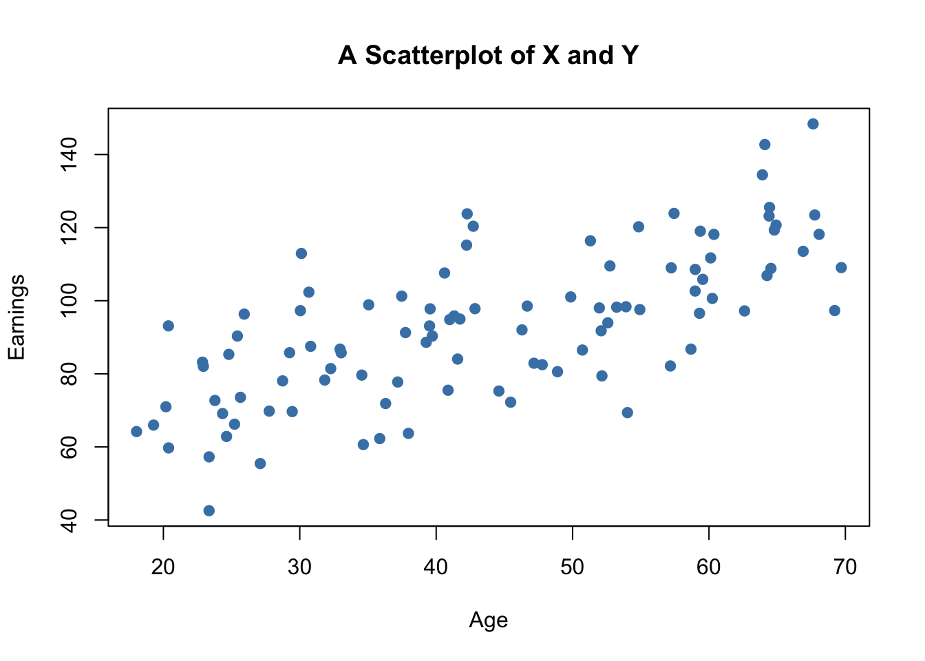
The plot shows positive correlation between age and earnings. This is in line with the notion that older workers earn more than those who joined the working population recently.
Sample Covariance and Correlation
By now you should be familiar with the concepts of variance and covariance. If not, we recommend you to work your way through Chapter 2 of the book.
Just like the variance, covariance and correlation of two variables are properties that relate to the (unknown) joint probability distribution of these variables. We can estimate covariance and correlation by means of suitable estimators using a sample \((X_i,Y_i)\), \(i=1,\dots,n\).
The sample covariance
\[ s_{XY} = \frac{1}{n-1} \sum_{i=1}^n (X_i - \overline{X})(Y_i - \overline{Y}) \]
is an estimator for the population variance of \(X\) and \(Y\) whereas the sample correlation
\[ r_{XY} = \frac{s_{XY}}{s_Xs_Y} \] can be used to estimate the population correlation, a standardized measure for the strength of the linear relationship between \(X\) and \(Y\). See Chapter 3.7 in the book for a more detailed treatment of these estimators.
As for variance and standard deviation, these estimators are implemented as R functions in the stats package. We can use them to estimate population covariance and population correlation of the artificial data on age and earnings.
# compute sample covariance of X and Y
cov(X, Y)
#> [1] 213.934

# compute sample correlation between X and Y
cor(X, Y)
#> [1] 0.706372

# an equivalent way to compute the sample correlation
cov(X, Y) / (sd(X) * sd(Y))
#> [1] 0.706372
The estimates indicate that \(X\) and \(Y\) are moderately correlated.
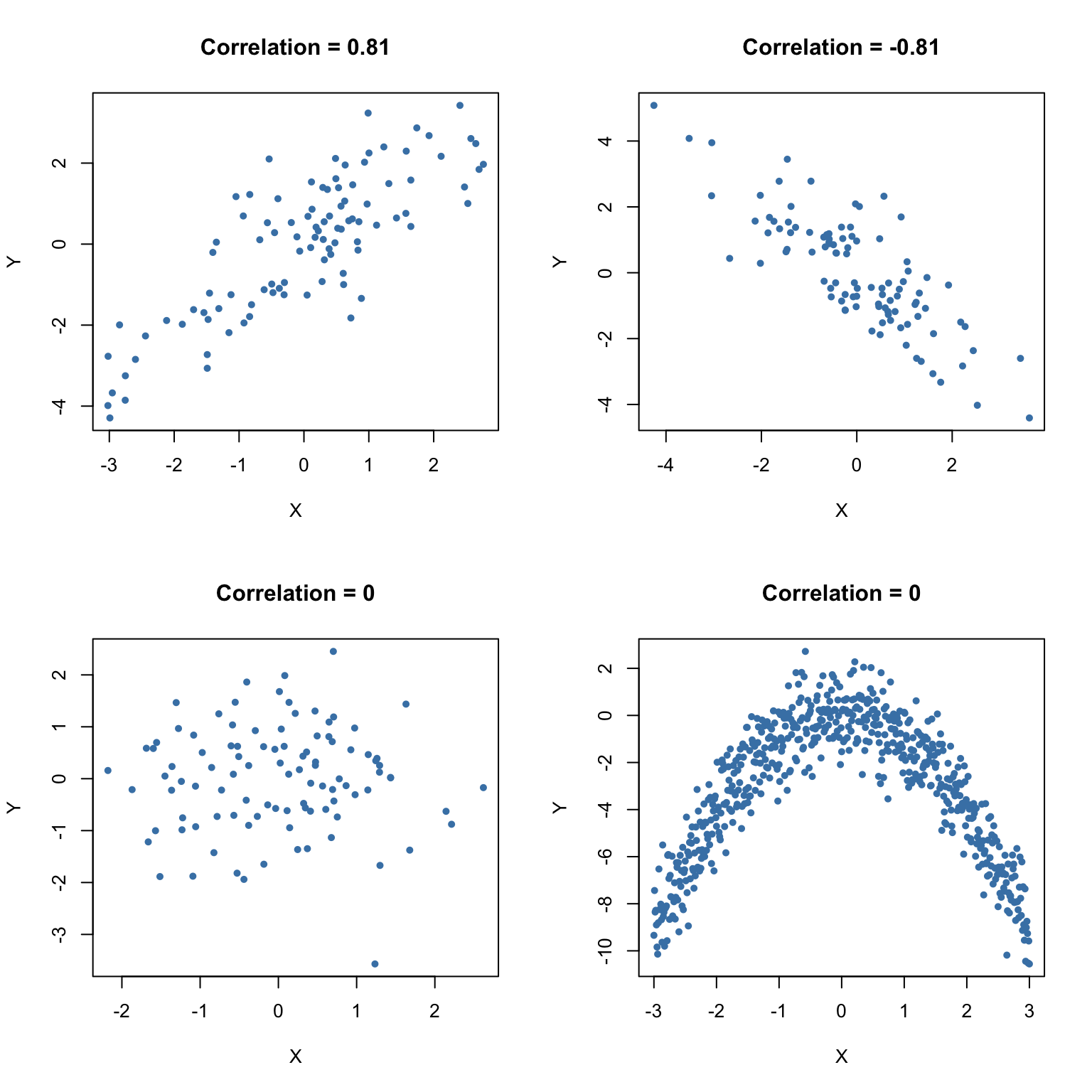
The next code chunk uses the function mvnorm() from package MASS (Ripley and Venables 2025) to generate bivariate sample data with different degrees of correlation.
library(MASS)

# set random seed
set.seed(1)

# positive correlation (0.81)
example1 <- mvrnorm(100,
                    mu = c(0, 0),
                    Sigma = matrix(c(2, 2, 2, 3), ncol = 2),
                    empirical = TRUE)

# negative correlation (-0.81)
example2 <- mvrnorm(100,
                    mu = c(0, 0),
                    Sigma = matrix(c(2, -2, -2, 3), ncol = 2),
                    empirical = TRUE)

# no correlation
example3 <- mvrnorm(100,
                    mu = c(0, 0),
                    Sigma = matrix(c(1, 0, 0, 1), ncol = 2),
                    empirical = TRUE)

# no correlation (quadratic relationship)
X <- seq(-3, 3, 0.01)
Y <- - X^2 + rnorm(length(X))

example4 <- cbind(X, Y)

# divide plot area as 2-by-2 array
par(mfrow = c(2, 2))

# plot datasets
plot(example1, col = "steelblue", pch = 20, xlab = "X", ylab = "Y",
     main = "Correlation = 0.81")

plot(example2, col = "steelblue", pch = 20, xlab = "X", ylab = "Y",
     main = "Correlation = -0.81")

plot(example3, col = "steelblue", pch = 20, xlab = "X", ylab = "Y",
     main = "Correlation = 0")

plot(example4, col = "steelblue", pch = 20, xlab = "X", ylab = "Y",
     main = "Correlation = 0")