8.1 A General Strategy for Modelling Nonlinear Regression Functions
Let us have a look at an example where using a nonlinear regression function is better suited for estimating the population relationship between the regressor, \(X\), and the regressand, \(Y\): the relationship between the income of schooling districts and their test scores.
# prepare the data
library(AER)
data(CASchools)
CASchools$size <- CASchools$students/CASchools$teachers
CASchools$score <- (CASchools$read + CASchools$math) / 2
We start our analysis by computing the correlation between both variables.
Here, income and test scores are positively related: school districts with above average income tend to achieve above average test scores. Does a linear regression function model the data adequately? Let us plot the data and add a linear regression line.
# fit a simple linear model
linear_model<- lm(score ~ income, data = CASchools)

# plot the observations
plot(CASchools$income, CASchools$score,
     col = "steelblue",
     pch = 20,
     xlab = "District Income (thousands of dollars)",
     ylab = "Test Score",
     cex.main = 0.9,
     main = "Test Score vs. District Income and a Linear OLS Regression Function")

# add the regression line to the plot
abline(linear_model,
       col = "red",
       lwd = 2)
legend("bottomright", legend="linear fit",lwd=2,col="red")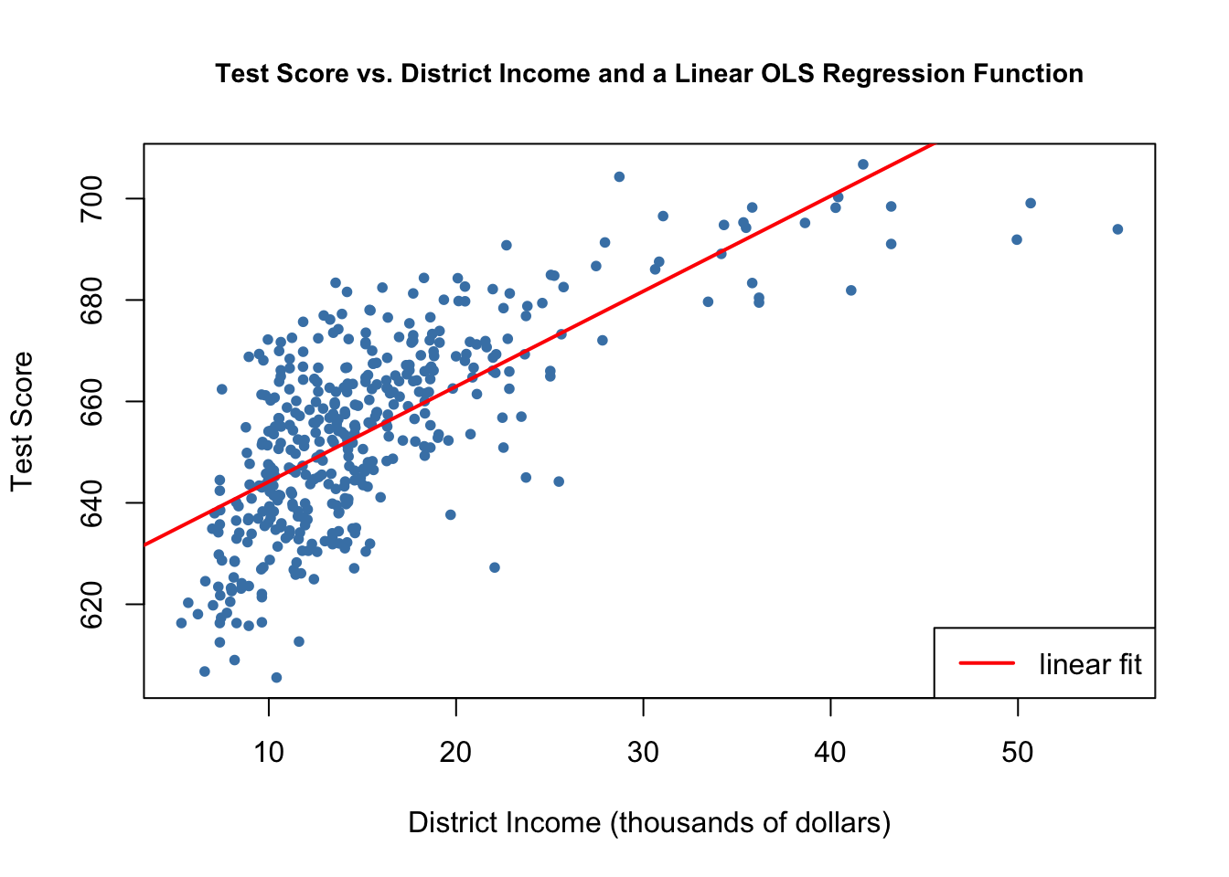
As pointed out in the book, the linear regression line seems to overestimate the true relationship when income is very high or very low and underestimates it for the middle income group.
Fortunately, OLS does not only handle linear functions of the regressors. We can, for example, model test scores as a function of income and the square of income. The corresponding regression model is
\[TestScore_i = \beta_0 + \beta_1 \times income_i + \beta_2 \times income_i^2 + u_i,\] called a quadratic regression model. That is, \(income^2\) is treated as an additional explanatory variable. Hence, the quadratic model is a special case of a multivariate regression model. When fitting the model with lm() we have to use the ^ operator in conjunction with the function I() to add the quadratic term as an additional regressor to the argument formula. This is because the regression formula we pass to formula is converted to an object of the class formula. For objects of this class, the operators +, -, * and ^ have a nonarithmetic interpretation. I() ensures that they are used as arithmetical operators, see ?I,
# fit the quadratic Model
quadratic_model <- lm(score ~ income + I(income^2), data = CASchools)

# obtain the model summary
coeftest(quadratic_model, vcov. = vcovHC, type = "HC1")
#>
#> t test of coefficients:
#>
#>                Estimate  Std. Error  t value  Pr(>|t|)
#> (Intercept) 607.3017435   2.9017544 209.2878 < 2.2e-16 ***
#> income        3.8509939   0.2680942  14.3643 < 2.2e-16 ***
#> I(income^2)  -0.0423084   0.0047803  -8.8505 < 2.2e-16 ***
#> ---
#> Signif. codes:  0 '***' 0.001 '**' 0.01 '*' 0.05 '.' 0.1 ' ' 1
The output tells us that the estimated regression function is
\[\widehat{TestScore}_i = \underset{(2.90)}{607.3} + \underset{(0.27)}{3.85} \times income_i - \underset{(0.0048)}{0.0423} \times income_i^2.\]
This model allows us to test the hypothesis that the relationship between test scores and district income is linear against the alternative that it is quadratic. This corresponds to testing
\[H_0: \beta_2 = 0 \ \ \text{vs.} \ \ H_1: \beta_2\neq0,\]
since \(\beta_2=0\) corresponds to a simple linear equation and \(\beta_2\neq0\) implies a quadratic relationship. We find that \(t=(\hat\beta_2 - 0)/SE(\hat\beta_2) = -0.0423/0.0048 = -8.81\) so the null is rejected at any common level of significance and we conclude that the relationship is nonlinear. This is consistent with the impression gained from the plot.
We now draw the same scatter plot as for the linear model and add the regression line for the quadratic model. Because abline() can only draw straight lines, it cannot be used here. lines() is a function which allows to draw nonstraight lines, see ?lines. The most basic call of lines() is lines(x_values, y_values) where x_values and y_values are vectors of the same length that provide coordinates of the points to be sequentially connected by a line. This makes it necessary to sort the coordinate pairs according to the X-values. Here we use the function order() to sort the fitted values of score according to the observations of income.
# draw a scatterplot of the observations for income and test score
plot(CASchools$income, CASchools$score,
     col  = "steelblue",
     pch = 20,
     xlab = "District Income (thousands of dollars)",
     ylab = "Test Score",
     main = "Estimated Linear and Quadratic Regression Functions")

# add a linear function to the plot
abline(linear_model, col = "green", lwd = 2)

# add quatratic function to the plot
order_id <- order(CASchools$income)

lines(x = CASchools$income[order_id],
      y = fitted(quadratic_model)[order_id],
      col = "red",
      lwd = 2)
legend("bottomright",legend=c("Linear Line","Quadratic Line"),
       lwd=2,col=c("green","red"))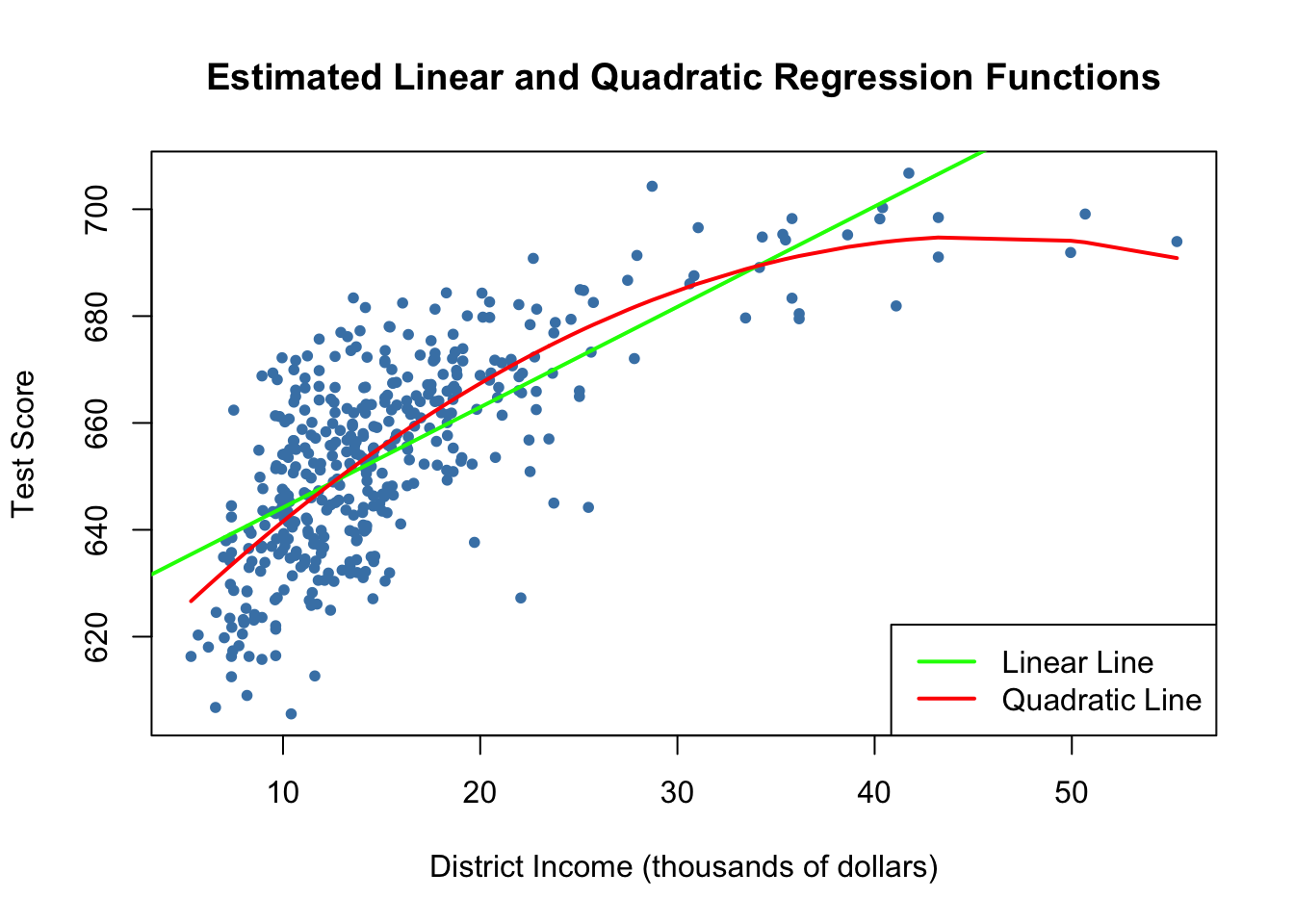
We see that the quadratic function does fit the data much better than the linear function.