4.1 Simple Linear Regression
To start with an easy example, consider the following combinations of average test score and the average student-teacher ratio in some fictional school districts.
To work with these data in R we begin by generating two vectors: one for the student-teacher ratios (STR) and one for test scores (TestScore), both containing the data from the table above.
# Create sample data
STR <- c(15, 17, 19, 20, 22, 23.5, 25)
TestScore <- c(680, 640, 670, 660, 630, 660, 635)

# Print out sample data
STR
#> [1] 15.0 17.0 19.0 20.0 22.0 23.5 25.0
TestScore
#> [1] 680 640 670 660 630 660 635
To build simple linear regression model, we hypothesize that the relationship between dependent and independent variable is linear, formally: \[ Y = b \cdot X + a. \] For now, let us suppose that the function which relates test score and student-teacher ratio to each other is \[TestScore = 713 - 3 \times STR.\]
It is always a good idea to visualize the data you work with. Here, it is suitable to use plot() to produce a scatterplot with STR on the \(x\)-axis and TestScore on the \(y\)-axis. Just call plot(y_variable ~ x_variable) whereby y_variable and x_variable are placeholders for the vectors of observations we want to plot. Furthermore, we might want to add a systematic relationship to the plot. To draw a straight line, R provides the function abline(). We just have to call this function with arguments a (representing the intercept)
and b (representing the slope) after executing plot() in order to add the line to our plot.
The following code reproduces Figure 4.1 from the textbook.
# create a scatterplot of the data
plot(TestScore ~ STR,ylab="Test Score",pch=20)

# add the systematic relationship to the plot
abline(a = 713, b = -3)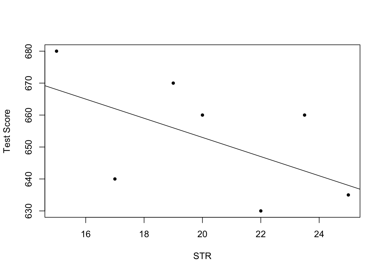
We find that the line does not touch any of the points although we claimed that it represents the systematic relationship. The reason for this is randomness. Most of the time there are additional influences which imply that there is no bivariate relationship between the two variables.
In order to account for these differences between observed data and the systematic relationship, we extend our model from above by an error term \(u\) which captures additional random effects. Put differently, \(u\) accounts for all the differences between the regression line and the actual observed data. Beside pure randomness, these deviations could also arise from measurement errors or, as will be discussed later, could be the consequence of leaving out other factors that are relevant in explaining the dependent variable.
Which other factors are plausible in our example? For one thing, the test scores might be driven by the teachers’ quality and the background of the students. It is also possible that in some classes, the students were lucky on the test days and thus achieved higher scores. For now, we will summarize such influences by an additive component:
\[ TestScore = \beta_0 + \beta_1 \times STR + \text{other factors}. \]
Of course this idea is very general as it can be easily extended to other situations that can be described with a linear model. Hence, the basic linear regression model we will work with is
\[ Y_i = \beta_0 + \beta_1 X_i + u_i. \]
Key Concept 4.1 summarizes the linear regression model and its terminology.
Key Concept 4.1
Terminology for the Linear Regression Model with a Single Regressor
The linear regression model is
\[Y_i = \beta_0 + \beta_1 X_i + u_i,\]
where
- the index \(i\) runs over the observations, \(i=1,\dots,n\);
- \(Y_i\) is the dependent variable, the regressand, or simply the left-hand variable;
- \(X_i\) is the independent variable, the regressor, or simply the right-hand variable;
- \(Y = \beta_0 + \beta_1 X\) is the population regression line also called the population regression function;
- \(\beta_0\) is the intercept of the population regression line;
- \(\beta_1\) is the slope of the population regression line;
- \(u_i\) is the error term.